Drifters in Hurricanes Fabian and Isabel, September 2003
Drifters
On September 3, 2003 eleven Minimet drifters were successfully deployed at a distance of about 18 hours in front of the projected path of a category-4 hurricane, Fabian, in the vicinity of 25°N, 65°W. Eight of them provided useful data: seven drifters transmitted data for about 5 months, one drifter for 1.5 months. SST, air pressure, ambient noise (to derive wind speed), wind direction, and position data have been analyzed. Wind directions are compared with scatterometer observations from SeaWinds on QuikSCAT and ADEOS-II (SWSA2).
Drifter measured ambient noise has been used to derive wind speed by calibrating against collocated scatterometer data.
Detailed comparisons are made for the passage of hurricanes Fabian and Isabel over or near the Minimet drifters.
Click on images for enlarged versions of plots.
Quality-controlled data files for 8 drifters are available for SST, air pressure, wind direction and wind
speed. Each data file contains interpolated drifter positions. Contact morzel@cora.nwra.com for access.
Latest file versions are called as follows: "NNNNN.dirpos", "NNNNN.pres10.pos", "NNNNN.speedpos01",
"NNNNN.sst09.pos"; for drifters 41578, 41581, 41582, 41583, 41584, 41585, 41587 and 41588.
Summary of Data
A summary of all drifter measured data (after quality control) is presented in the following table: Pos = position,
Pres = air pressure, SST = sea surface temperature, Dir = wind direction, Noise = acoustic noise
(to derive speed), Min = last date when all sensors were still working, Days = number of days corresponding
to Min.
Table 1.1: Summary of all Drifter Data
| | Ending Dates | | | Number of Obs |
| Drifter | Pos | Pres | SST | Dir | Noise | Min | Days | Pos | Pres | SST | Dir | Noise |
| | | | | | | |
| | | | | |
| 41578 | 2/07 | 2/03 | 2/06 | 2/02 | 2/06 | 2/02 |
151 | 1098 | 6879 | 1744 | 6951 | 6846 |
| 41581 | 2/04 | 2/04 | 2/04 | 2/04 | 2/04 | 2/04 |
154 | 1147 | 6965 | 1747 | 6926 | 6934 |
| 41582 | 2/04 | 2/02 | 2/04 | 2/04 | 2/04 | 2/02 |
152 | 1309 | 7272 | 1836 | 7326 | 7310 |
| 41583* | 10/24 | 10/04 | 10/25 | 10/25 | 10/22 | 10/04 |
30 | 105 | 1177 | 375 | 1477 | 1415 |
| 41584 | 2/14 | 2/11 | 2/06 | 2/13 | 2/13 | 2/06 |
155 | 1231 | 7335 | 1861 | 7404 | 7406 |
| 41585 | 1/22 | 1/13 | 1/22 | 1/22 | 1/22 | 1/13 |
132 | 1038 | 6061 | 1599 | 6352 | 6261 |
| 41587 | 2/25 | 2/23 | 2/25 | 2/25 | 1/09 | 1/09 |
129 | 1311 | 7884 | 1998 | 7948 | 5999 |
| 41588 | 1/30 | 1/28 | 1/30 | 1/30 | 1/30 | 1/28 |
146 | 1151 | 6417 | 1714 | 6808 | 6811 |
| | | | | | | |
| | | | | |
| av days* | | | | | | |
146 |
| Nobs/day* | | | | | | |
| 8 | 46 | 11 | 46 |
45 |
* Note: Drifter 41583 is not included in the averages.
During each successful data transmission, drifters usually report four 15-min averages from the last
hour for pressure, direction, and acoustic noise. SST gets reported only once, from the last 15 min.
So on average, there are about 11 transmissions per day, with about 8 successful positionings per day.
The daily sampling frequency is quite complex, and depends mostly on successful communications
with the ARGOS network. The sampling pattern for drifter 41578 is depicted in Figures 1.0 a&b, which
are representative of all drifters. Note, that after day 310 (11/6/2003), there start to be
sampling gaps between 8-12 and 19-23 UTC, corresponding to local times of 3-7am and 2-6pm.
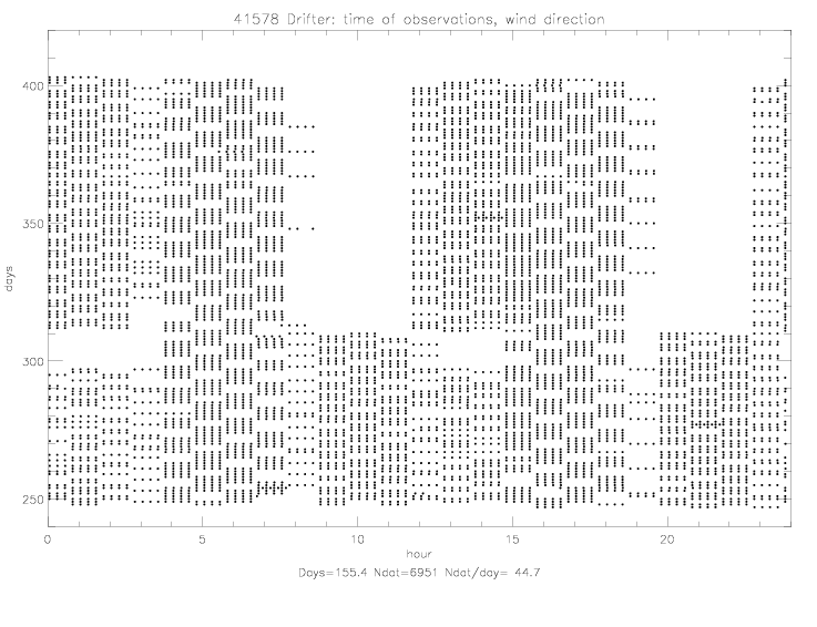
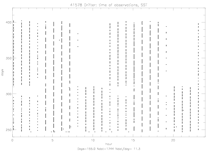 Fig. 1.0 Sampling from drifter 41578, for (a) wind direction, and (b) SST.
1. Drifter Tracks
Below are plots of eight drifter tracks: 41578, 41581, 41582, 41583 (stops after 51 days: 9/3-10/24/03), 41584, 41585, 41587, and 41588. All data have been processed. On average, for each drifter there are about 8 position
data per day, except for drifter 41583 which has only about 2 positions per day. Every day is indicated with a black dot (interpolated in time), every 10 days are marked in red and labeled. For quality control, all instances when the drift velocity exceeded 100 cm/s are marked with small red numbers. None of those were eliminated because they do not seem to indicate large erratic movement of the drifters. For collocation purposes, the drifter locations will be compared with satellite observations that have a resolution of only 25km x 25km.
Three pairs of drifters were deployed in close vicinity to each other, and some of them followed similar paths for several days. The three pairs are: 41578 & 41585, 41581 & 41583, and 41584 & 41588. In the following pictures, the latitude and longitude limits are chosen so that the resolution and lon/lat ratio is the same for all plots.
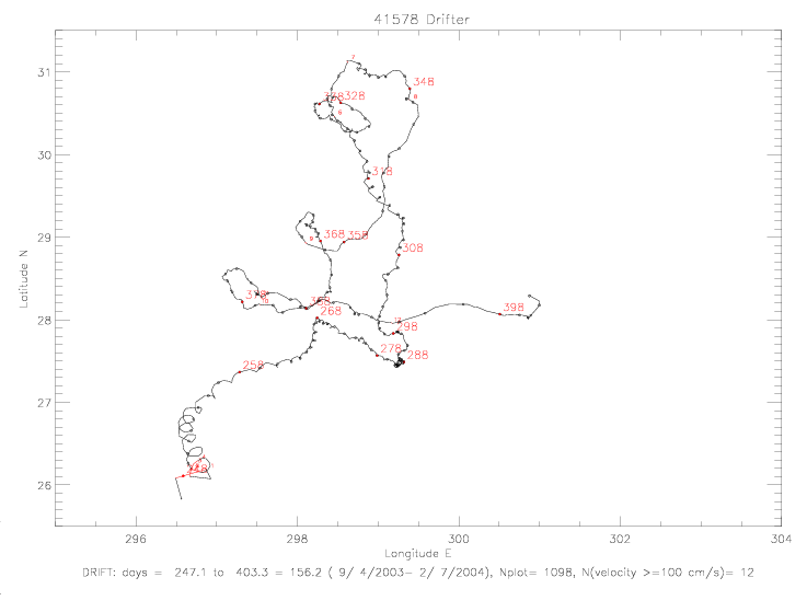
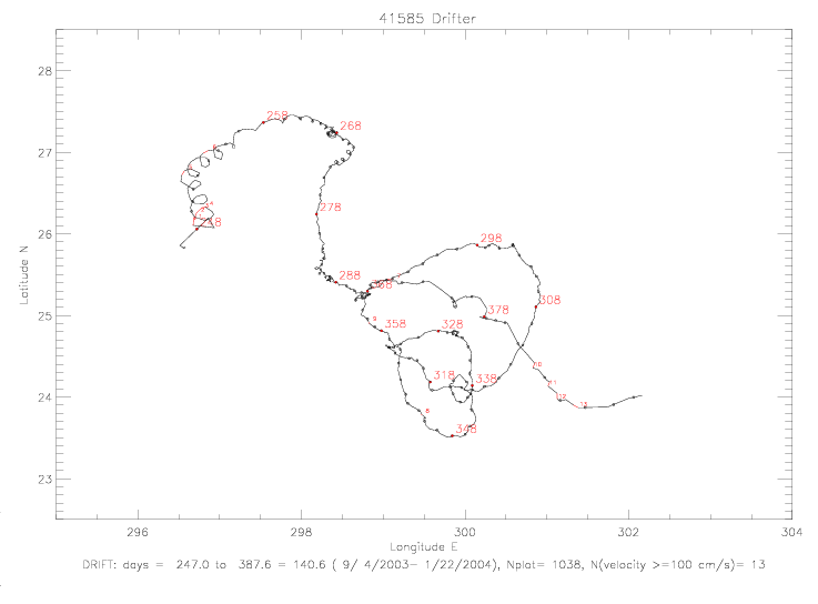 Fig. 1.1 (a) Drifter 41578, and (b) Drifter 41585.
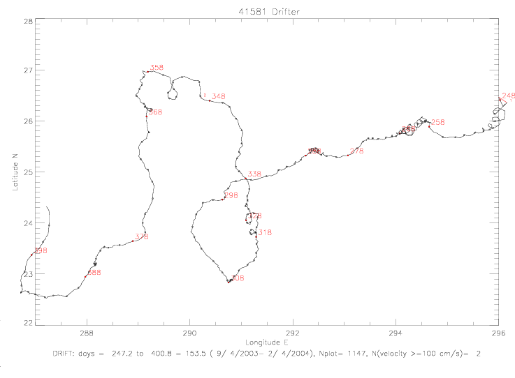
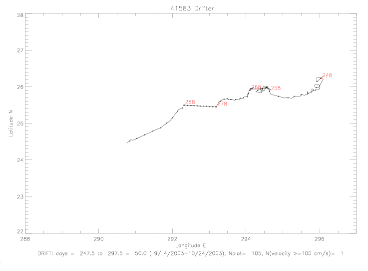 Fig. 1.2 (a) Drifter 41581, and (b) Drifter 41583.
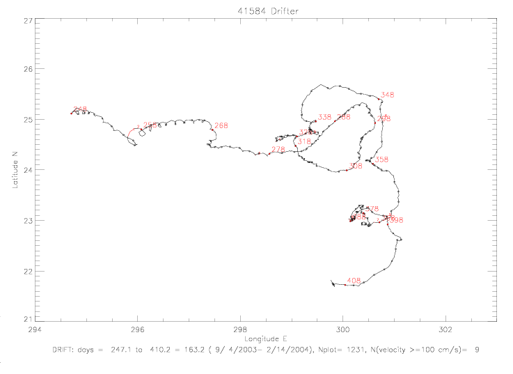
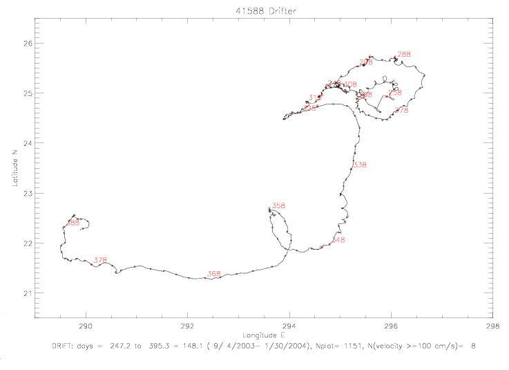 Fig. 1.3 (a) Drifter 41584, and (b) Drifter 41588.
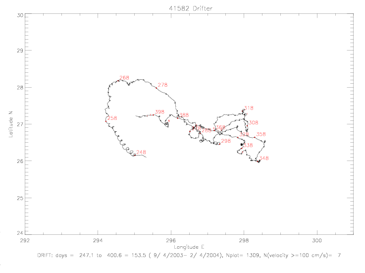
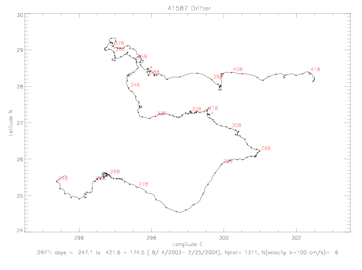 Fig. 1.4 (a) Drifter 41582, and (b) Drifter 41587.
2. Drifter Tracks and Track of Hurricane Fabian
In the plots below, drifter tracks are shown relative to hurricane locations. Open squares indicate starting positions, and solid
dots are the last reported positions. The data time period for each drifter is provided below the
the plots, in days starting on 1/1/2003.
The track of the hurricane is indicated by
two different data sets. The red track (with crosses at data locations) is from NOAA's preliminary
Tropical Cyclone Report (for reference, see
Unisys' 2003 Hurricane/Tropical Data for Atlantic). Those location data are available about every 3 hours.
They are labeled with the day in September, hr Z, and the reported wind speed (in m/s). The blue track,
with diamonds, indicates approximate hurricane locations inferred from SeaWinds swaths. At those locations, the time
is in days in 2003, hr:min Z; satellite names (QSCAT or SWSA2),\ and revolution number are also provided. In addition,
there are lines plotted connecting the SeaWinds hurricane center locations with NOAA centers, interpolated to the
SeaWinds time. Plots of the surface wind field provided by these satellite swaths are provided further below on
this page.
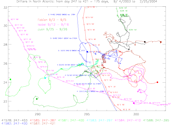 Fig.2.1 Drifter tracks for 9/4/2003 to 1/6/2004 (124 days).
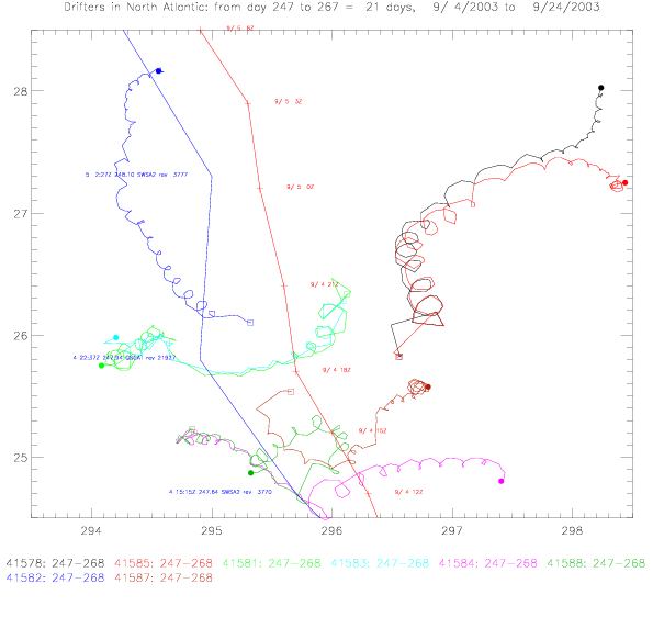
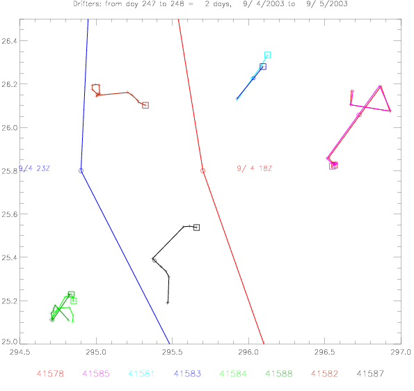 Fig.2.2 (a) Drifter tracks for the first 20 days, and (b) the first 2 days.
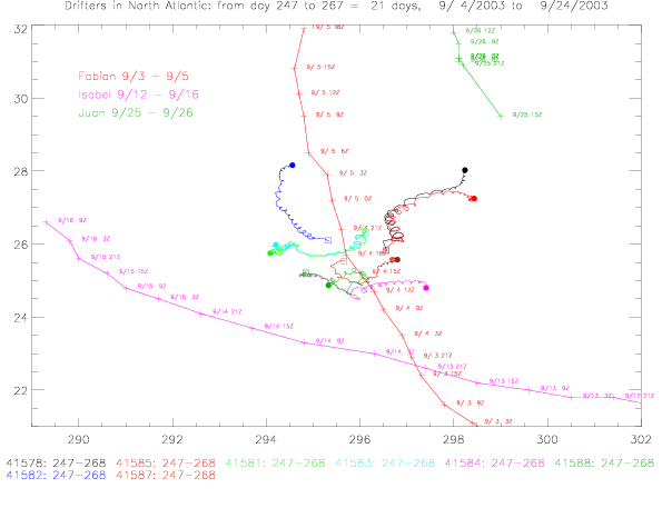 Fig.2.3 Drifter tracks for the first 20 days, and paths of hurricanes Fabian, Isabel, and Juan.
3.a. Satellite Winds and Hurricane Fabian
The scatterometer overflight data swaths in the area of the drifters during Fabian, a category-4 hurricane with
maximum winds of 64m/s, are presented below. The data come from SeaWinds on QSCAT and SeaWinds on ADEOS-II (SWSA2).
Each satellite measured the center of the hurricane about every 7
revolutions, i.e. every 11:47 hr (except after the first rev, when the next two revs missed the center). The coverage of the
two satellites in the area of interest is almost identical: QSCAT's swath area is shifted by only 1° to the west of SWSA2's
swath. QSCAT follows SWSA2 7:20 hr later. The more recently deployed SWSA2 instrument has been tuned to perform as close
to QSCAT measurements as possible.
Drifter observations are shown (with blue vectors), when there were observations within 60min of the satellite data.
The time differences (drifter-scatterometer) are indicated below the figures. These preliminary plots do not include
any drifter wind speed data (inferred from measured ambient noise). In thses plots the drifter wind vectors are drawn
with a speed of 20m/s.
The satellite data are either from ascending tracks (Southeast to Northwest, e.g. SWSA2 3741 and QSCAT 21898) or
descending tracks (Northeast to Southwest, e.g. SWSA2 3763 and QSCAT 21820).
Also plotted are the hurricane centers inferred from the scatterometer wind vectors (black crosses) and the
time-interpolated hurricane centers from NOAA (red crosses). Those locations are used to plot the hurricane tracks in
Figures 2.1 and 2.2. Note, that in almost all cases the scatterometer locations are to the Southwest of the NOAA locations.
Both scatterometers employ a rain detection algorithm that is based on the radar backscatter signal.
Rainflagged vectors are plotted in red and green. Previous analysis has indicated that the
rain effect is diminished above wind speeds of 15m/s. Rain-flagged vectors with speeds of less than 15m/s are plotted in red,
vectors with speeds &ge 15m/s are plotted in green. It appears, however, from these figures that for many wind vector cells
(WVC) the rain-flagged vectors fit nicely into the surrounding non-flagged wind field. The rain-effect is most strongly
observed north of the hurricane center where the wind vectors appear to be more East-West than expected. Those erroneous
directions are due to the rain effect on the radar backscatter which tends to align wind vectors in a cross-track direction.
It is also apparent that the
abrupt (seemingly non-physical) change in the measured flow field to the Northwest of the hurricane center seems to
be caused by the rain effect: in this area the scatterometer wind vectors turn abruptly from a East-West direction to
a North-South direction. The same blocky flow happens to the Southwest of the hurricane center, but not quite as badly as
Northwest of the center. There are instances, however, when the the circular nature of the wind field around the
hurricane center is quite well represented by the scatterometer measurements, see e.g. QSCAT rev 21948, SWSA2 3791, and
QSCAT 21927.
The maximum windspeeds measured by the scatterometers are much less than NOAA's reported maximum speeds for the hurricane,
as indicated on the figures. On average, the reported maximum wind speeds are 16m/s smaller for QSCAT, and 19m/s smaller
for SWSA2.
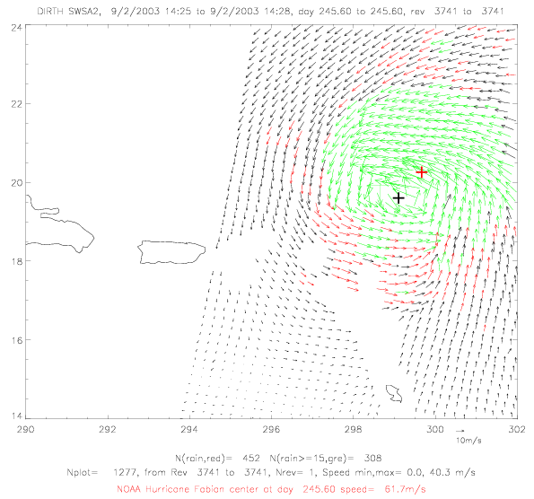
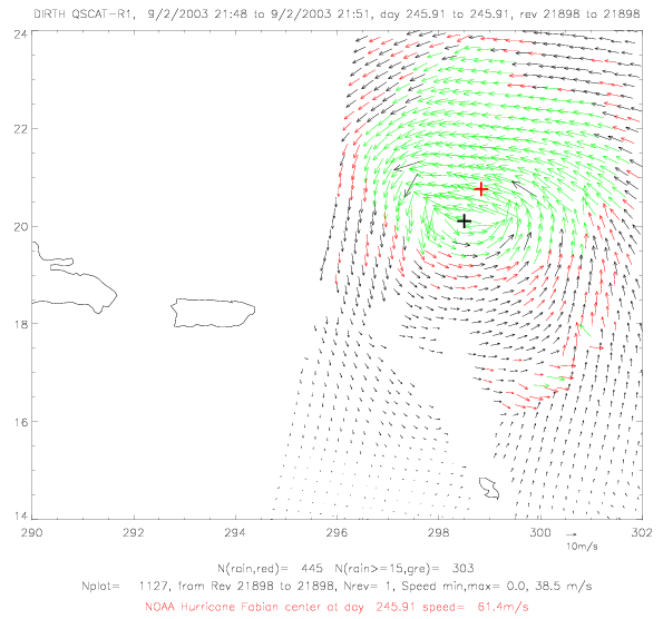 Fig. 3.1 (a) SWSA2 rev 3741 on 9/2/2003 at 14:25, and (b) QSCAT rev 21898 at 21:41.
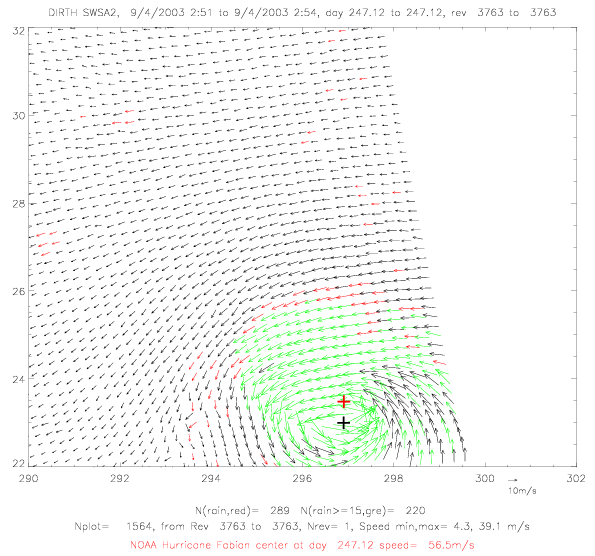
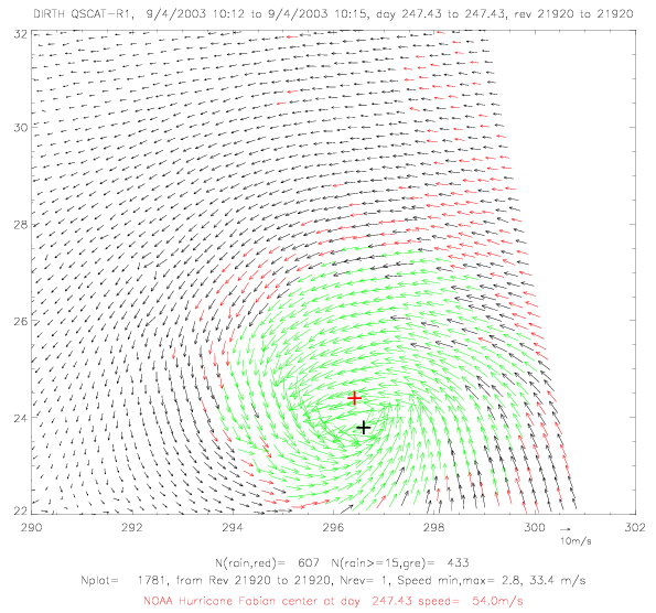 Fig. 3.2 (a) SWSA2 rev 3763 on 9/4/2003 at 2:51, and (b) QSCAT rev 21920 at 10:15.
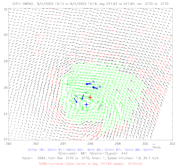
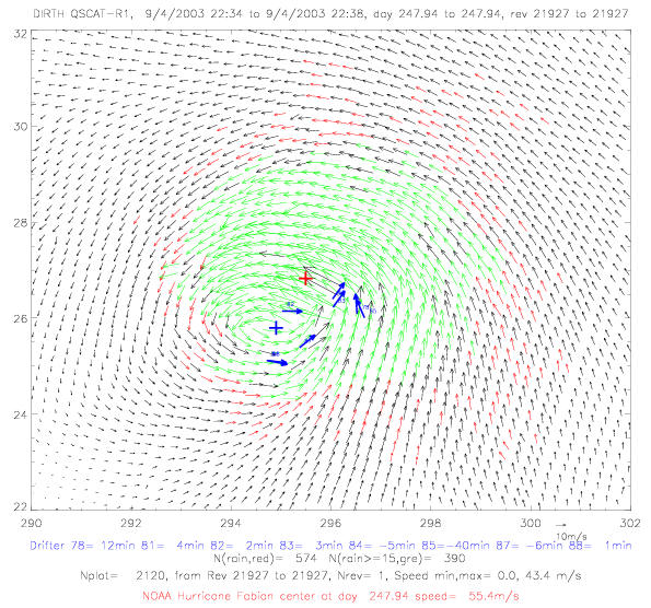 Fig. 3.3 (a) SWSA2 rev 3770 on 9/4/2003 15:13, and (b) QSCAT rev 21927 at 22:34.
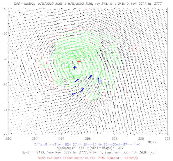
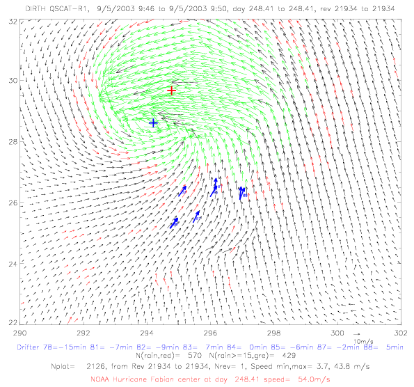 Fig. 3.4 (a) SWSA2 rev 3777 on 9/5/2003 at 2:25, and (b) QSCAT rev 21934 at 9:46.
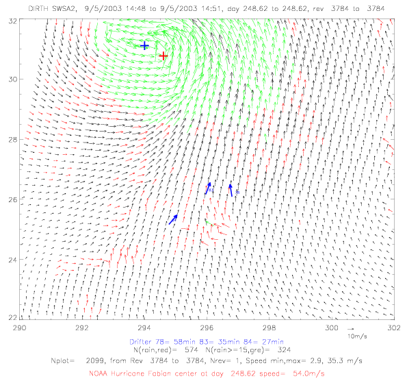
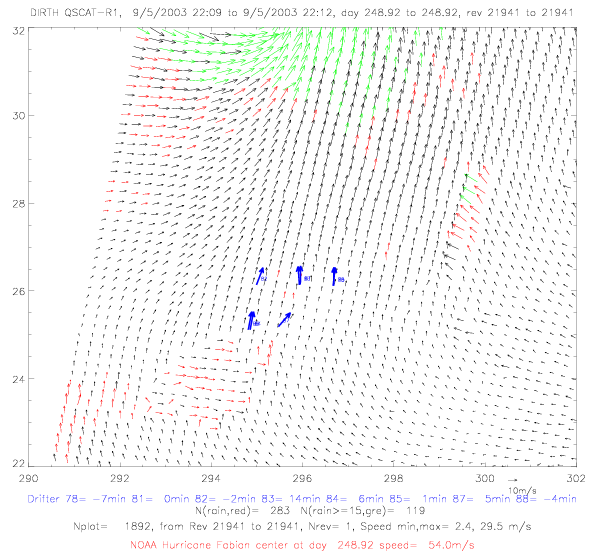 Fig. 3.5 (a) SWSA2 rev 3784 on 9/5/2003 at 14:47, and (b) QSCAT rev 21941 at 22:07.
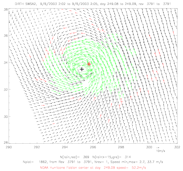
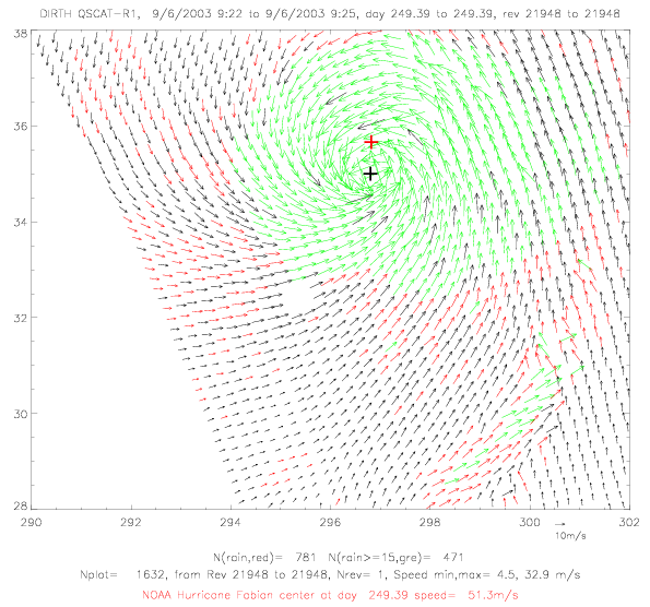 Fig. 3.6 (a) SWSA2 rev 3791 on 9/6/2003 at 2:02, and (b) QSCAT rev 21948 at 9:22.
3.b. Satellite Winds and Hurricane Isabel
During the time period of 9/12 to 9/18/2003 the category-5 hurricane Isabel (with maximum wind speeds of 72m/s) crossed
the North Atlantic very close to the deployed drifters. Collocated wind vector plots are presented below. The plots are
similar to the fabian plots, except that there are no scatterometer inferred hurricane centers, i.e.
there are no black crosses marking these locations. It appears that the scatterometer derived wind fields indicate
hurricane centers very close to the centers identified by NOAA (red crosses).
From drifter-to-drifter comparisons (see Fig. 6.15a), it has become clear that the wind direction measurements on drifter
41583 are not error free. It appears that there is an offset that grows over time. When compared with the nearby
deployed drifter 41581, this offset has been determined to be 7.9° for days 247-252.4. It is 14.3° for days
252.4-258, and 32.4° for days 258-267. The original measurements from drifter 41583 are drawn in magenta, and the
corrected directions are plotted in light blue. The correction amounts to a counter-clockwise rotation of about 8-32°.
Drifter 41583 appears in 15 plots with wind vectors from QSCAT and ADEOS-II. Assuming that the scatterometer wind
fields are close to truth (in the vicinity of the difters), the corrected 41583 wind directions are a better match in
12 cases, are about the same in 2 cases, and look worse in only one case.
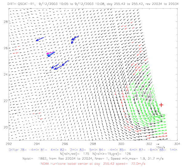
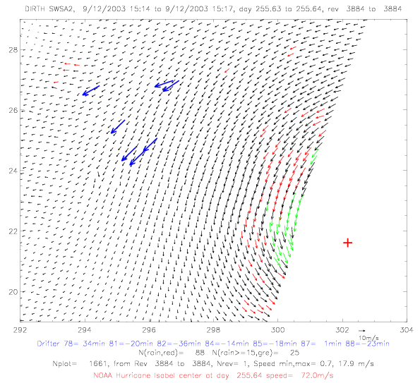 Fig. 3.7 (a) QSCAT rev 22034 on 9/12/2003 at 10:08, and (b) SWSA2 rev 3884 at 15:17.
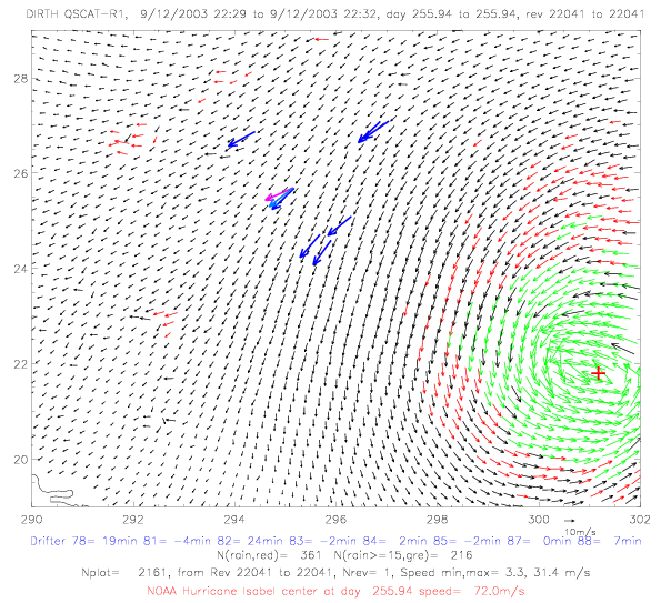
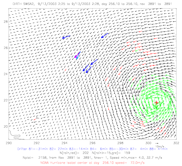 Fig. 3.8 (a) QSCAT rev 22041 on 9/12/2003 at 22:32, and (b) SWSA2 rev 3891 on 9/13 at 2:28.
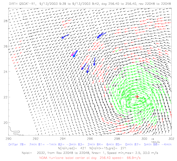
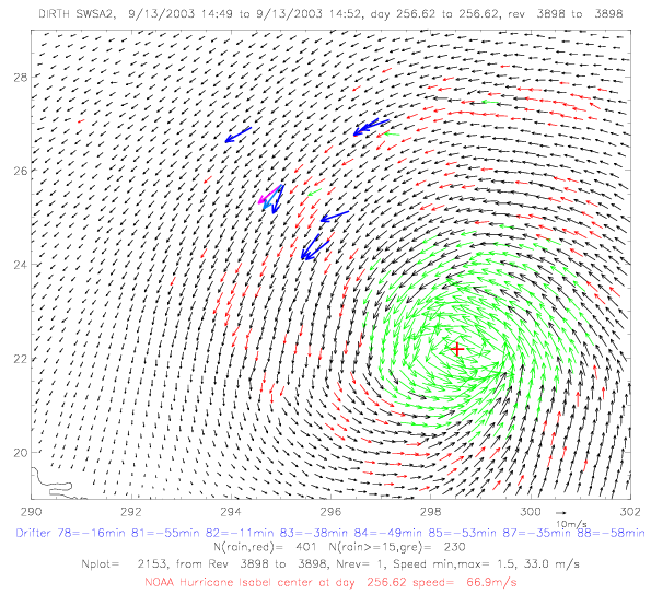 Fig. 3.9 (a) QSCAT rev 22048 on 9/13/2003 at 9:39, and (b) SWSA2 rev 3898 at 14:49.
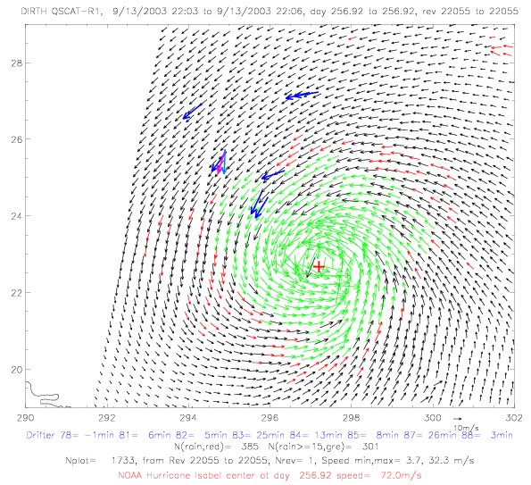
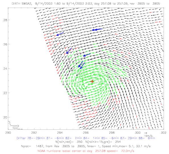 Fig. 3.10 (a) QSCAT rev 22055 on 9/13/2003 at 22:03, and (b) SWSA2 rev 3905 on 9/14 at 2:00.
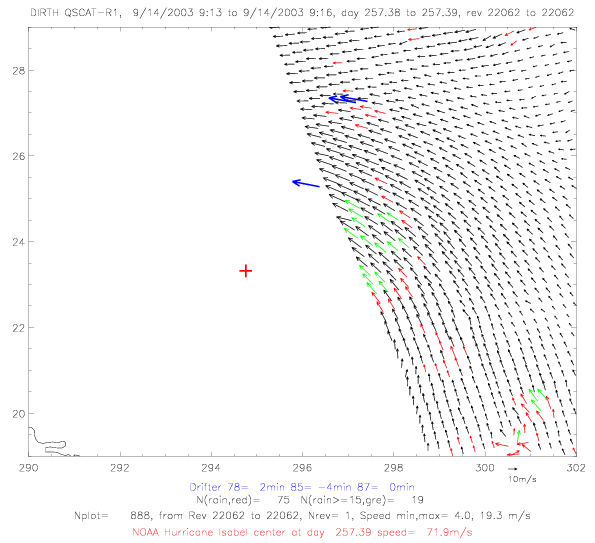
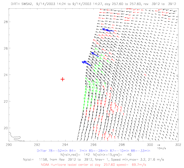 Fig. 3.11 (a) QSCAT rev 22062 on 9/14/2003 at 9:13, and (b) SWSA2 rev 3912 at 14:24.
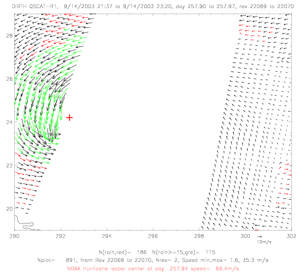
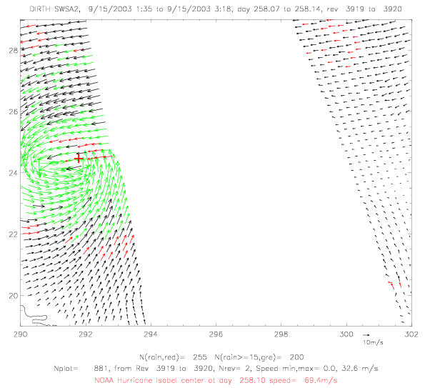 Fig. 3.12 (a) QSCAT revs 22069 & 22070 on 9/14/2003 at 21:37-23:20, and
(b) SWSA2 revs 3919 & 3920 on 9/15 at 1:35-3:18.
Fig. 3.12 (a) QSCAT revs 22069 & 22070 on 9/14/2003 at 21:37-23:20, and
(b) SWSA2 revs 3919 & 3920 on 9/15 at 1:35-3:18.
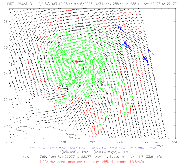
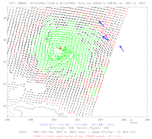 Fig. 3.13 (a) QSCAT rev 22077 on 9/15/2003 at 10:28, and (b) SWSA2 rev 3927 at 15:39.
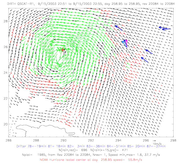
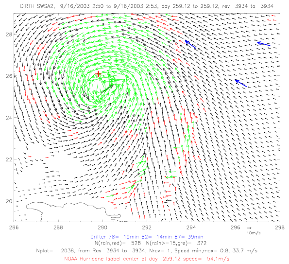 Fig. 3.14 (a) QSCAT rev 22084 on 9/15/2003 at 22:51, and (b) SWSA2 rev 3934 on 9/16 at 2:50.
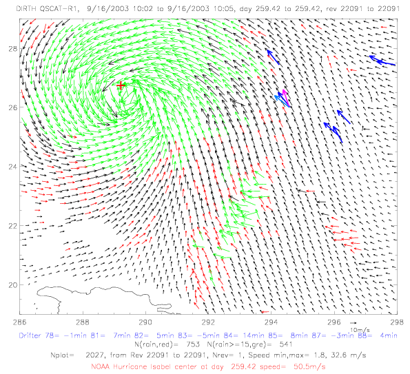
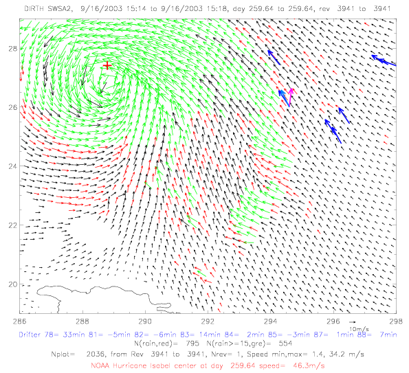 Fig. 3.15 (a) QSCAT rev 22091 on 9/16/2003 at 10:02, and (b) SWSA2 rev 3941 at 15:14.
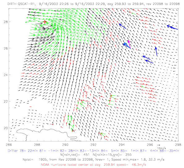
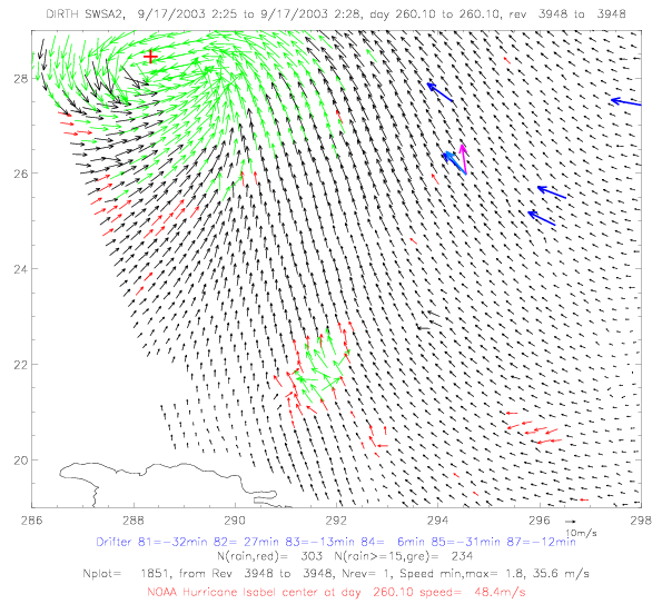 Fig. 3.16 (a) QSCAT rev 22098 on 9/16/2003 at 22:26, and (b) SWSA2 rev 3948 on 9/17 at 2:25.
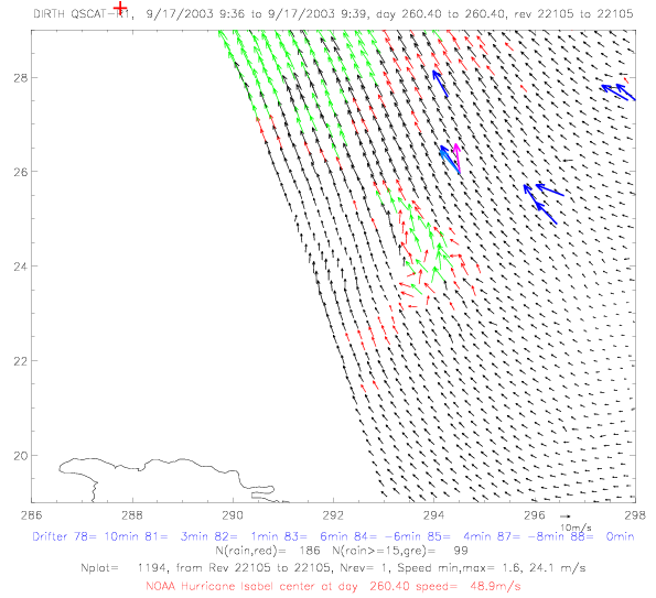
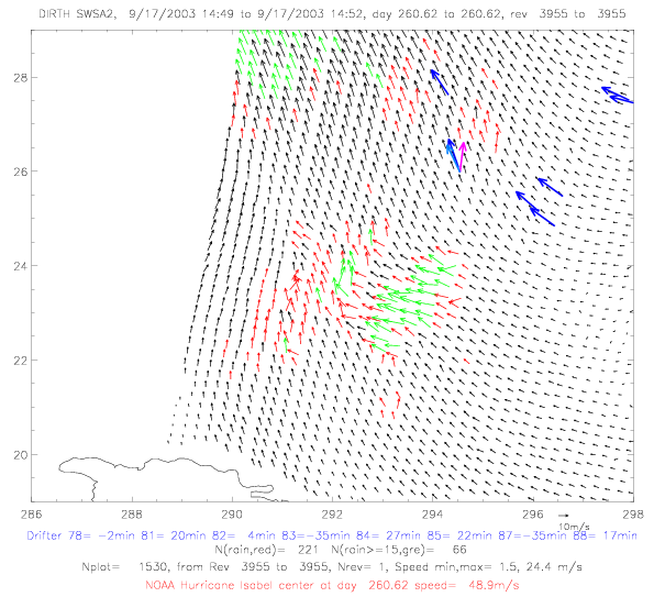 Fig. 3.17 (a) QSCAT rev 22105 on 9/17/2003 at 9:36, and (b) SWSA2 rev 3955 at 14:49.
4. Drifter Air pressure
All drifter measured air pressure data have been processed. On average, for each drifter
there are about 46 air pressure observations per day. Whenever a contact is made with ARGOS, the most recent 4
selected values (from four 15min measuring intervals) are transmitted for pressure (as well as for wind direction and
acoustic noise). For SST, only the most recent value is sent. That means for pressure (and wind direction and speed),
about every other hour is sampled continuously for four 15min intervals.
- Sampling Frequency : Air pressure is sampled 4 times per hour, at 1Hz for 160sec. Sampling
begins at 9, 24, 39, and 54min past the hour in drifter time, which is not the same as real time.
- Measurement and Selection / Averaging : The 160 pressure measurements are stored, and a median is taken of
the lowest 10 values. A second median is then taken from values that are within +/- 1mb of the first median.
This is done to eliminate positive only pressure spikes from the data set. This median is transmitted
to ARGOS. All available ARGOS data are collected by Pacific Gyre ("SQL" data).
- Quality Control at CoRA : The SQL data files have been retrieved from Pacific Gyre (excluding
records with 850mb), N read, and were processed as follows:
- All records with times that are within 5min of each other and with the same pressure values were
eliminated (N repeat).
- There were also many records within 5min of each other but with different pressure data. Those have been
manually edited to eliminate erroneous data spikes (N elim).
- Finally, there still remained a few spikes in the data files that were deleted in the final step of the
quality control (N bad). An example of those spikes is presented below for drifter 41578 (Fig. 4.1).
Table 4.1: Pressure Quality Control (statistics for first 112 days)
| Drifter | N read | N repeat | N elim | N bad | N plot |
| 41578 | 9501 | 4425 | 168 | 15 | 4893 |
| 41581 | 20778 | 15437 | 389 | 11 | 4941 |
| 41582 | 26325 | 20729 | 303 | 6 | 5287 |
| 41583 | 2083 | 1064 | 60 | 28 | 931 |
| 41584 | 22739 | 17332 | 330 | 1 | 5076 |
| 41585 | 22375 | 16934 | 421 | 11 | 5009 |
| 41587 | 20580 | 15153 | 388 | 13 | 5026 |
| 41588 | 20907 | 15922 | 287 | 27 | 4671 |
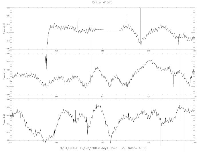 Fig. 4.1 Air Pressure 41578, pre-quality control first 112 days, including "Nbad" spikes.
Six drifters were released in pairs and are plotted next to each other: 41578 & 41585, 41581 & 41583, and 41584 & 41588.

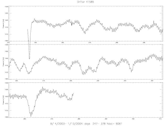 Fig. 4.2 (a) Air Pressure 41578 and (b) 41585.
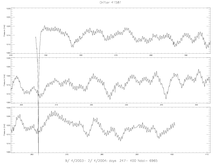
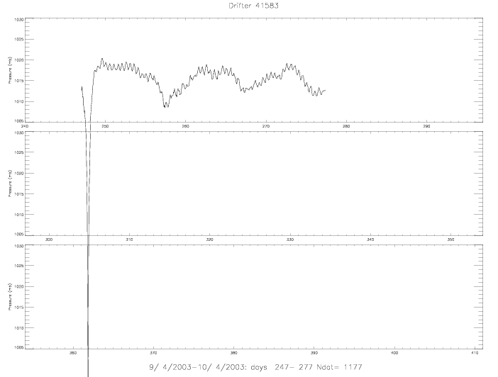 Fig. 4.3 (a) Air Pressure 41581 and (b) 41583.
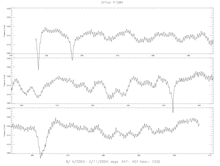
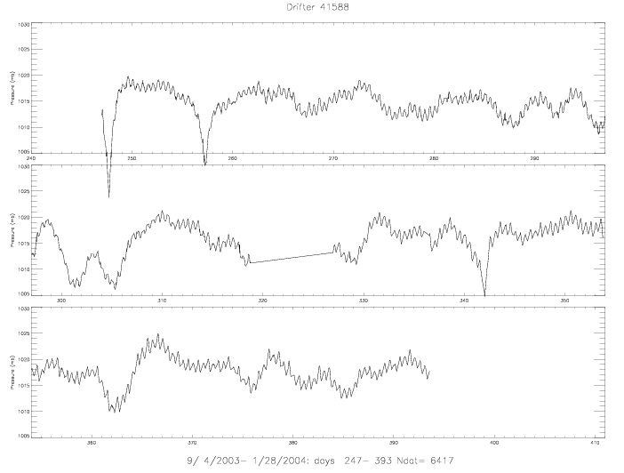 Fig. 4.4 (a) Air Pressure 41584 and (b) 41588.
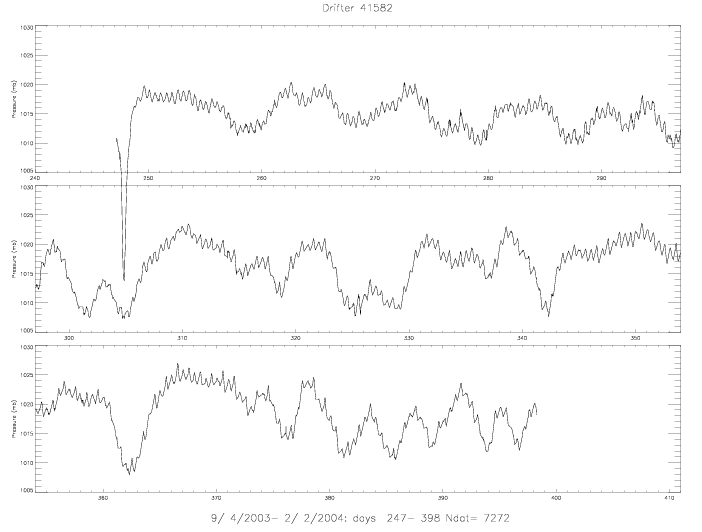
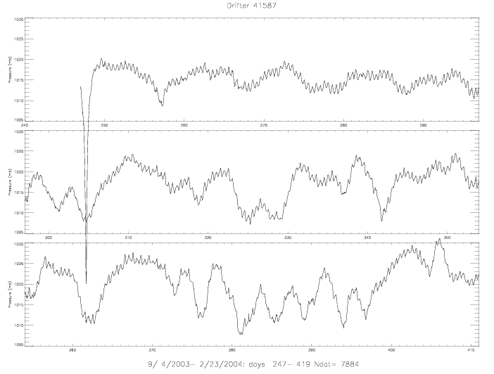 Fig. 4.5 (a) Air Pressure 41582 and (b) 41587.
Intercomparison of all air pressure data shows that drifter 41585 needs to adjusted by subtracting 1mb.
This has been done for the final data release ("41585.pres10.pos").
5. Drifter Sea Surface Temperature
On average, for each drifter there are about 11 SST observations per day, or about one every 2 hours.
- Sampling Frequency : SST is sampled every minute as an instantaneous measurement.
- Measurement and Selection / Averaging : Every 15min the 15 SST values are averaged, and
the most recent average is transmitted to ARGOS.
- Quality Control at CoRA : The SQL data files have been retrieved from Pacific Gyre (exlcuding records
&le -5°C), N read , and were processed as follows:
- All SST values < 15°C were eliminated (N min), as were all records with times that are within 5min
of each other and with the same SST values (N repeat).
- There were also many records within 5min of each other but with different SST data. Those have been
manually edited to eliminate erroneous data spikes (N elim).
- Finally, there still remained a few spikes in the data files that were deleted in the final step of the
quality control (N bad). An example of those spikes is presented below for drifter 41578 (Fig. 5.1).
Table 5.1: SST Quality Control (statistics for first 118 days)
| Drifter | N read | N min | N repeat | N elim | N bad | N plot |
| 41578 | 2513 | 4 | 1210 | 7 | 7 | 1285 |
| 41581 | 5501 | 13 | 4152 | 29 | 4 | 1303 |
| 41582 | 6910 | 4 | 5496 | 17 | 5 | 1388 |
| 41583 | 678 | 3 | 353 | 6 | 0 | 316 |
| 41584 | 5986 | 3 | 4603 | 46 | 3 | 1331 |
| 41585 | 5865 | 6 | 4502 | 39 | 1 | 1317 |
| 41587 | 5436 | 4 | 4073 | 34 | 1 | 1324 |
| 41588 | 5956 | 11 | 4596 | 27 | 3 | 1319 |
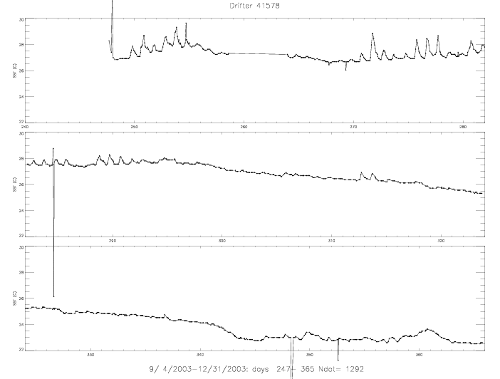 Fig. 5.1 SST 41578, pre-quality control, first 118 days, including "Nbad" spikes.
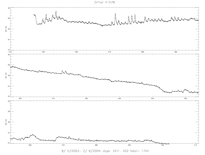
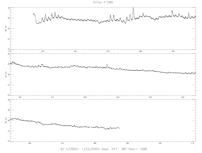 Fig. 5.2 (a) SST 41578, and (b) SST 41585.
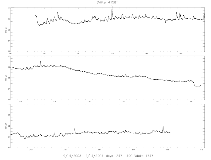
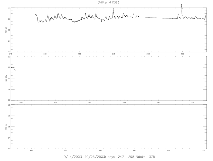 Fig. 5.3 (a) SST 41581 and (b) 41583.
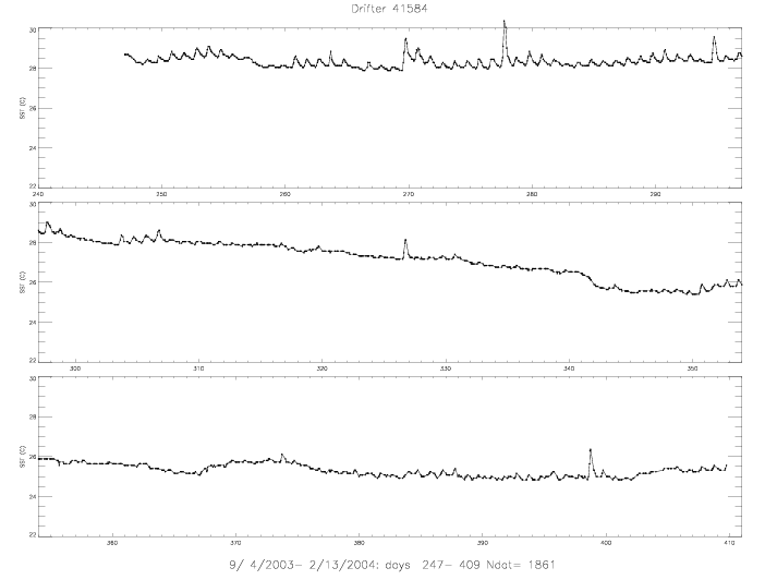
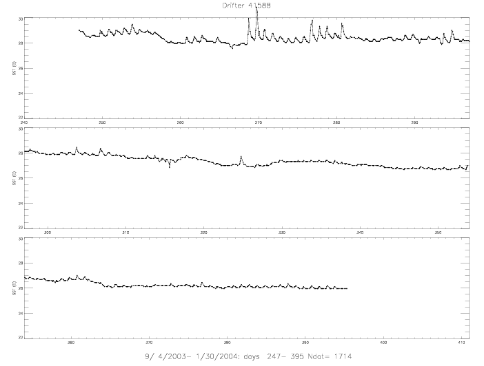 Fig. 5.4 (a) SST 41584 and (b) 41588.
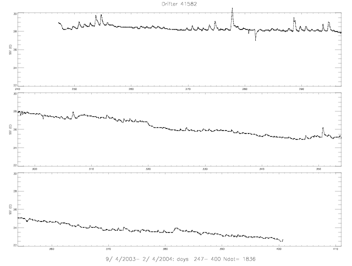
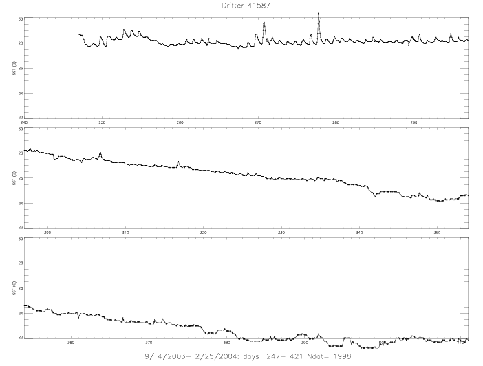 Fig. 5.5 (a) SST 41582 and (b) 41587.
5.a SST immediately after hurricane Fabian
The following plots examine SST during passage of hurricane Fabian and for several days
afterwards. The hurricane produces a cooling of the SST, and this cooling persists
for at least seven days in the wake of the hurricane trail.
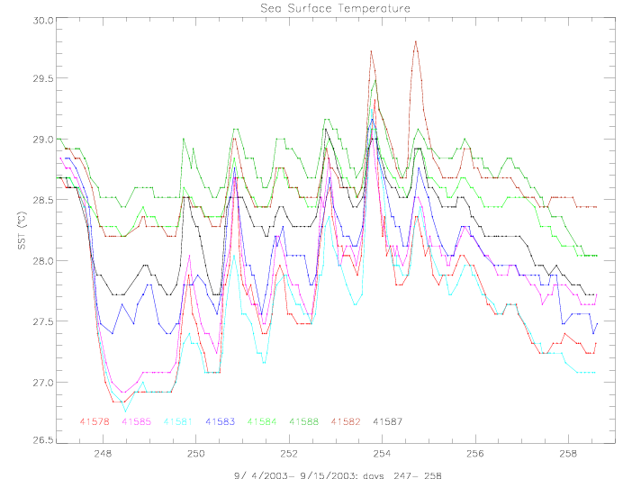 Fig. 5.6 SST of eight drifters during the first eleven days.
Three pairs of drifters stay relatively close together for several days after
the passage of the hurricane. In the drifter plot below, the coloring scheme is the same as
in Fig. 5.6 for SST. Every day is marked with a small circle. Day 250 is labeled.
Also indicated is the track of hurricane Fabian.
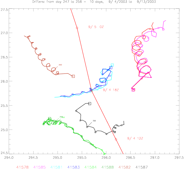 Fig. 5.7 Drifter tracks during the first 10 days after deployment (squares mark start of tracks).
The SST measurements of three pairs of drifters are illustrated below. The three pairs are
41578 & 41585, 41581 & 41583, and 41584 & 41588. The top panel shows SST measurements when
recorded within 30min by both drifters.
The difference is shown in the middle panel (with the 2-day average of the difference
superimposed in red). The bottom panel depicts the distance between the drifters (in km),
with the 2D tracks superimposed. Squares mark the deployment locations.
The North & East vectors indicate geographic orientation, and provide a 20km scale length
for the tracks. On the 2D tracks every 5 days are labeled (on the black tracks); the
corresponding day on the red track is marked with a red dot only.
The 41581&41583 pair remained within 50km of each other for 50 days, when
drifter 41583 stopped reporting data. The data for this pair is presented in two figures:
for the first 30 days, and also for the entire 50 day record.
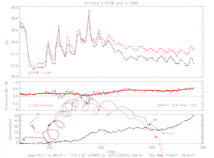
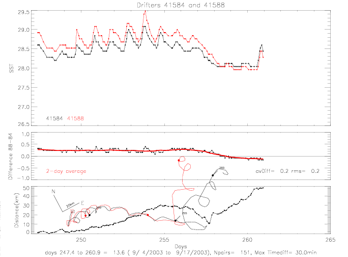 Fig. 5.8 SST of nearby drifters: (a) 41578 & 41585, and (b) 41584 & 41588.
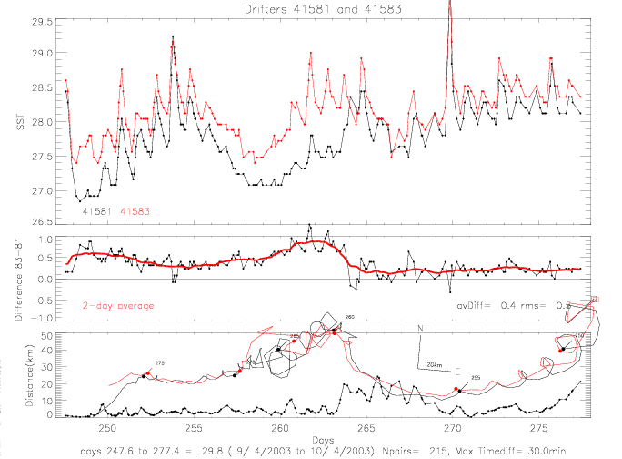
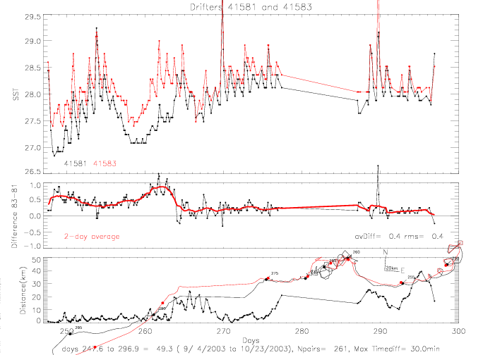 Fig. 5.9 SST of nearby drifters 41581 & 41583: (a) first 30 days, and (b) 50 days.
Relatively constant temperature differences between nearby drifters might indicate erroneous
offsets of some or all instruments. Drifter 41585 is about 0.2°C warmer than 41578,
until day 252.5, when the drifters are starting to move further apart than 5km.
SST from drifter 41588 is a relatively constant 0.25°C warmer than 41584, up to a distance of
30km on day 257, when the drifters are starting to move into different directions.
The relationship between 41583 and 41581 is a little more complicatead. The two drifters
stay within 20km for the entire data record of 41583, but the temperature difference
between the two records changes from ca. 0.5°C during the first 11 days (days 247-259)
to 0.2 °C during the last 32 days of drifter 41583 (days 265-297). Note that the largest
diurnal SST change observed by both drifters (at day 270), of about 3.5°C, is
measured by both drifters within 0.4°C.
In order to illustrate the SST cooling from the hurricane, and the slow warming of
SST in the wake of the hurricane, the 2-day averaged SST are plotted below for the first 11 days.
Fig. 5.10a shows the 2-day averages for all drifters. In Fig. 5.10b nearby drifters have been averaged.
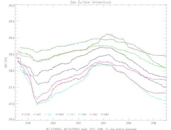
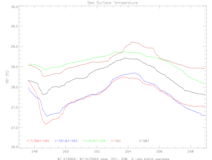 Fig. 5.10 2-day averaged SST: from (a) all drifters, and (b) averaged pairs.
To illustrate the geographic pattern of SST changes relative to the track of the Fabian, the 2-day
averaged SST data are plotted vs. distance from the track and vs. time, for the first 7 days
after the hurricane passes through the deployment array.
Fig. 5.11a shows (SST-27) for all drifters. This figure shows how close several drifters stayed
to each other during the first week of measurements. In fig.5.11b nearby drifter pairs have
been averaged. It becomes apparent that the largest cooling occurs to the right of the
hurricane track, of at least 1.5°C. To the left of the track the cooling amounts to only
0.6°C.
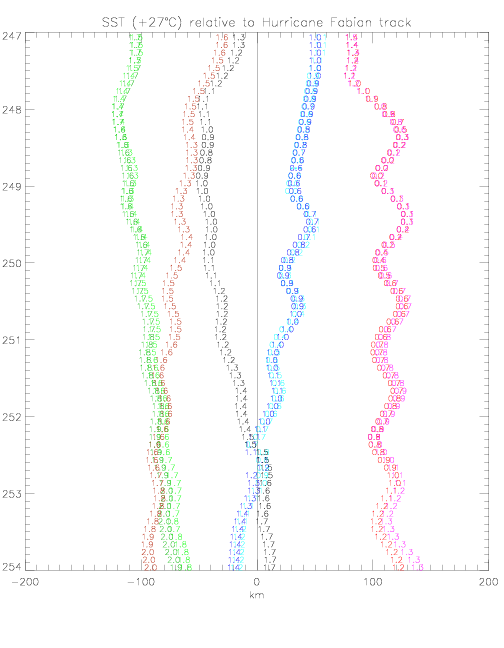
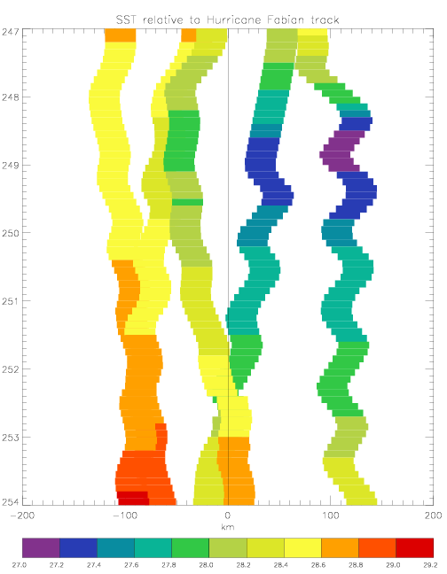 Fig. 5.11 2-day averaged SST relative to hurricane track: from (a) all drifters (SST-27),
and (b) averaged pairs.
Fig. 5.11 2-day averaged SST relative to hurricane track: from (a) all drifters (SST-27),
and (b) averaged pairs.
6. Drifter Wind direction
On average, for each drifter there are about 46 wind direction observations per day. As in the case of pressure,
that corresponds to 4 measurements (sampling an hour continuously for four 15min averaging intervals) about
every other hour.
- Sampling Frequency : Wind direction is sampled at the same time as pressure, i.e. 4 times per hour,
at 1Hz for 160sec. Sampling begins at 9, 24, 39, and 54min past the hour in drifter time.
- Measurement and Selection / Averaging : The 160 compass values are sorted into 5° bins.
The bin with the greatest number of samples is taken as the wind direction value and transmitted to ARGOS.
- Quality Control at CoRA : The SQL data files have been retrieved from Pacific Gyre, N read ,
and were processed as follows:
- All initial 0° values were eliminated (N 0), as were all values greater than 360°.
(N 360), and all records with times that are within 5min of each other and with the same dir values
(N repeat).
- There were also many records within 5min of each other but with different dir data. Those have been
manually edited to eliminate erroneous data spikes (N elim).
- A correction for the magnetic declination of -14° was applied to the compass measured directions.
And the directions were changed from meteorological ("blowing from") to oceanographic ("blowing to")
directions (as are the scatterometer data); i.e. a direction of 90° means a wind blowing from west to east.
Drifter 41577 recorded wind directions for only 1.5 hr on September 4.
Table 6.1: Wind Direction Quality Control (statistics for first 124 days)
| Drifter | N read | N 0 | N 360 | N repeat | N elim | N plot |
| 41578 | 10684 | 156 | 36 | 5023 | 91 | 5379 |
| 41581 | 23180 | 176 | 56 | 17323 | 227 | 5398 |
| 41582 | 28952 | 176 | 43 | 22770 | 185 | 5778 |
| 41583 | 2812 | 76 | 12 | 1401 | 61 | 1262 |
| 41584 | 25156 | 204 | 69 | 19135 | 213 | 5535 |
| 41585 | 24572 | 168 | 77 | 18541 | 316 | 5470 |
| 41587 | 23052 | 148 | 90 | 16981 | 312 | 5521 |
| 41588 | 24948 | 144 | 72 | 19040 | 200 | 5492 |
| 41577 | 96 | 68 | 0 | 16 | 4 | 8 |
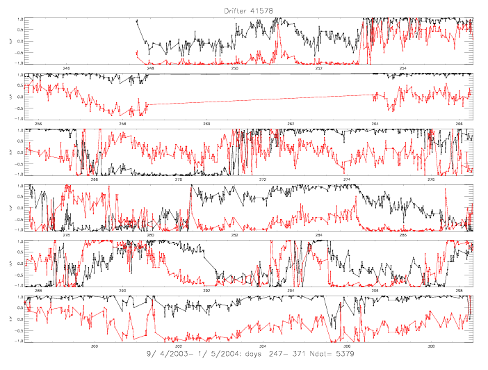
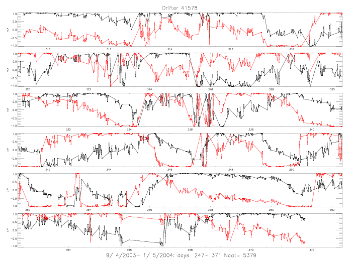 Fig. 6.1 U (black) and V (red) components of wind directions from 41578.
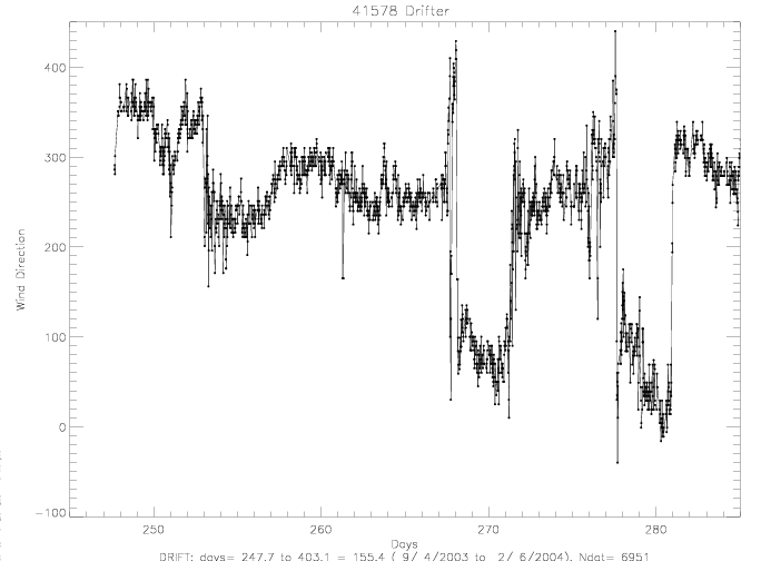
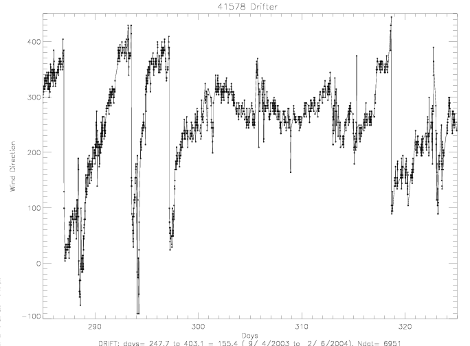 Fig. 6.2 Wind direction from drifter 41578, (a) days 245-285, and (b) days 285-325.
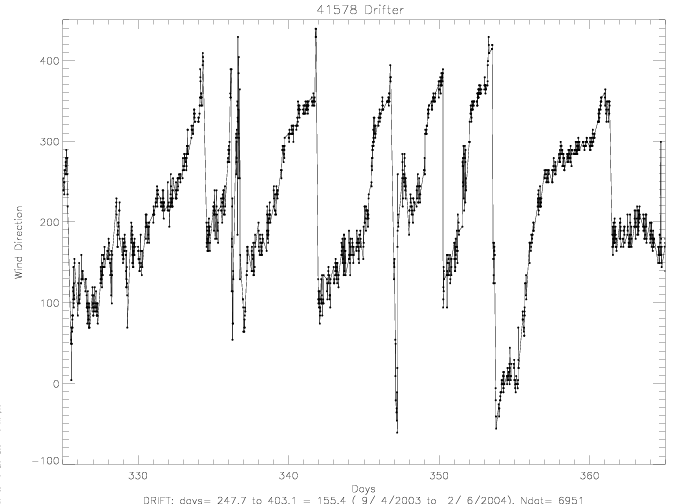
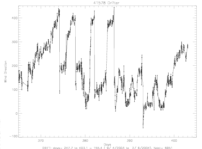 Fig. 6.3 Wind direction from drifter 41578, (a) days 325-365, and (b) days 365-405.
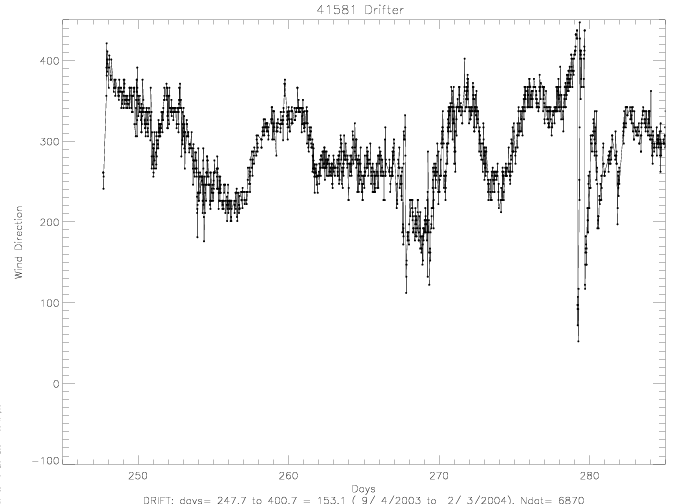
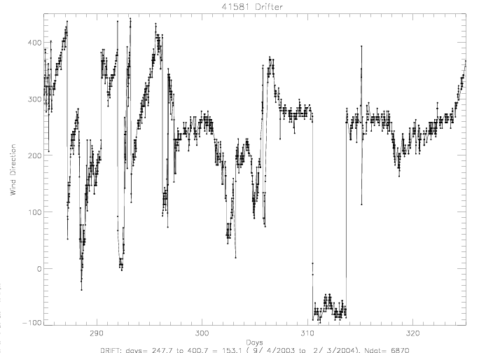 Fig. 6.4 Wind direction from drifter 41581, (a) days 245-285, and (b) days 285-325.
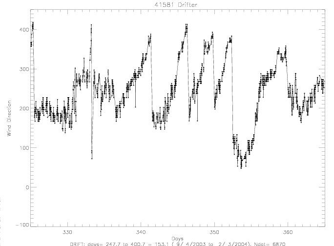
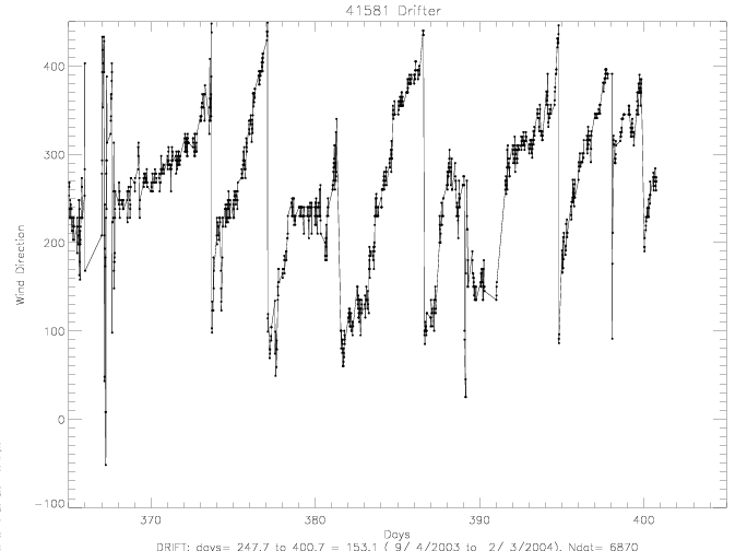 Fig. 6.5 Wind direction from drifter 41581, (a) days 325-365, and (b) days 365-405.
6.a Collocated Scatterometer wind directions
In the following figures, the 1-hourly averaged drifter wind directions are plotted with collocated QSCAT and ADEOS-II
scatterometer data (black solid dots) for the first 14 days. Rain-flagged scatterometer are marked with open
squares.
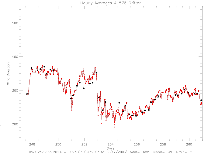
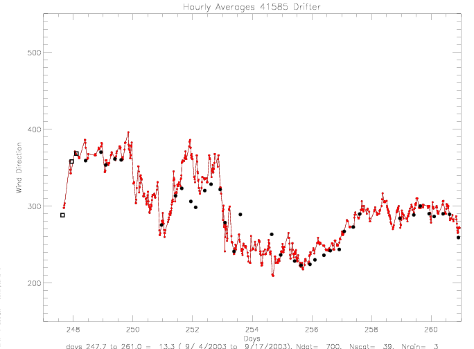 Fig. 6.6 1-hourly averaged wind directions, for drifters (a) 41578, and (b) 41585.
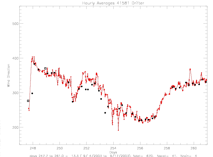
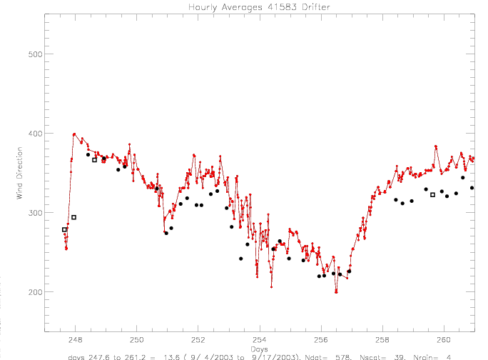 Fig. 6.7 1-hourly averaged wind directions, for drifters (a) 41581, and (b) 41583.
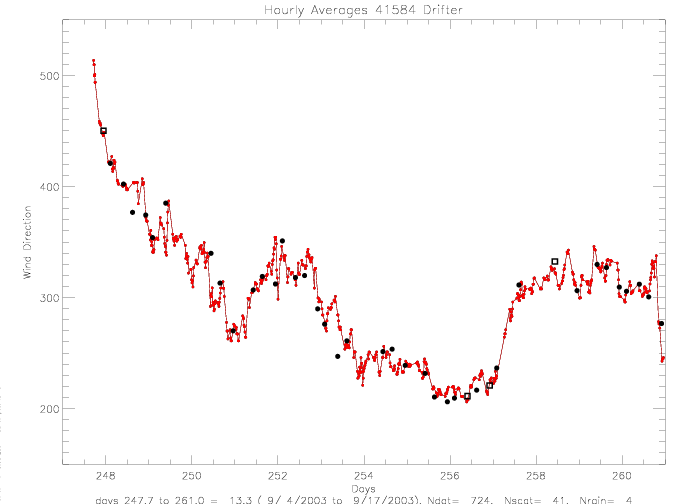
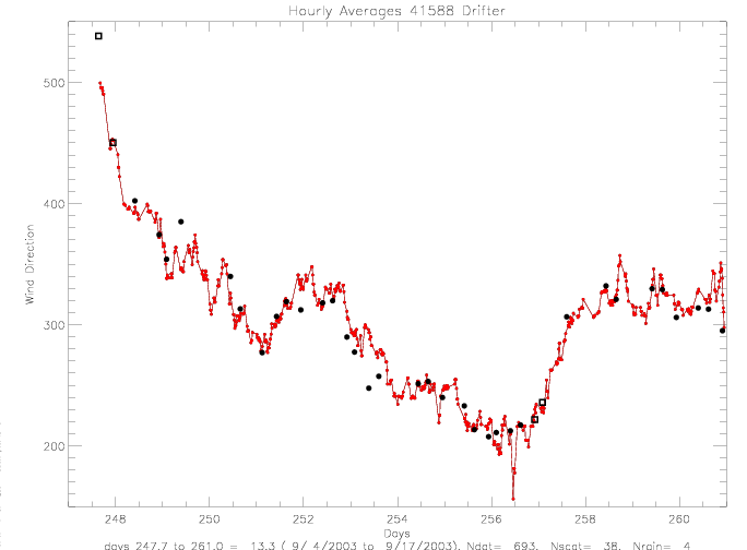 Fig. 6.8 1-hourly averaged wind directions, for drifters (a) 41584, and (b) 41588.
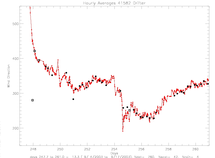
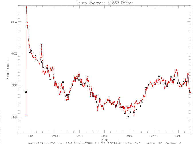 Fig. 6.9 1-hourly averaged wind directions, for drifters (a) 41582, and (b) 41587.
Below are presented scatterplots of collocated drifter and scatterometer wind direction observations.
Any pair of observations within 1hr and 100km are allowed. On average, the separation was 12-19km and 3-9min.
All rain-flagged scatterometer data are marked in red. The dashed lines indicate the rms of the
data around the 1:1 fit (for the no-rain data only).
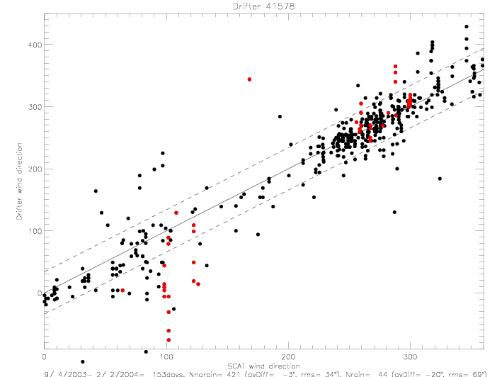
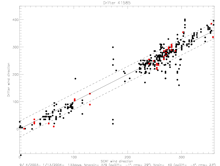 Fig. 6.10 Drifter vs. scatterometer wind directions, for drifters (a) 41578, and (b) 41585.
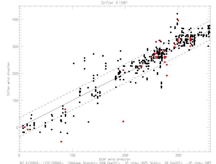
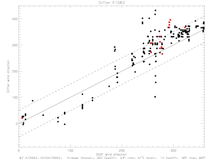 Fig. 6.11 Drifter vs. scatterometer wind directions, for drifters (a) 41581, and (b) 41583.

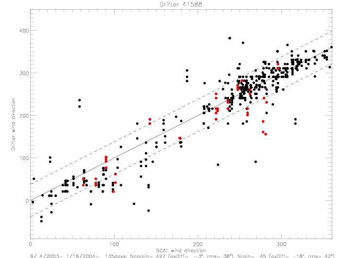 Fig. 6.12 Drifter vs. scatterometer wind directions, for drifters (a) 41584, and (b) 41588.
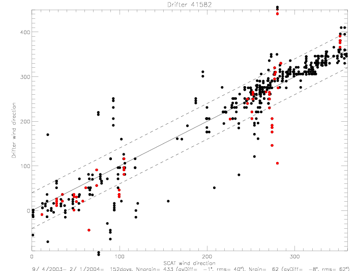
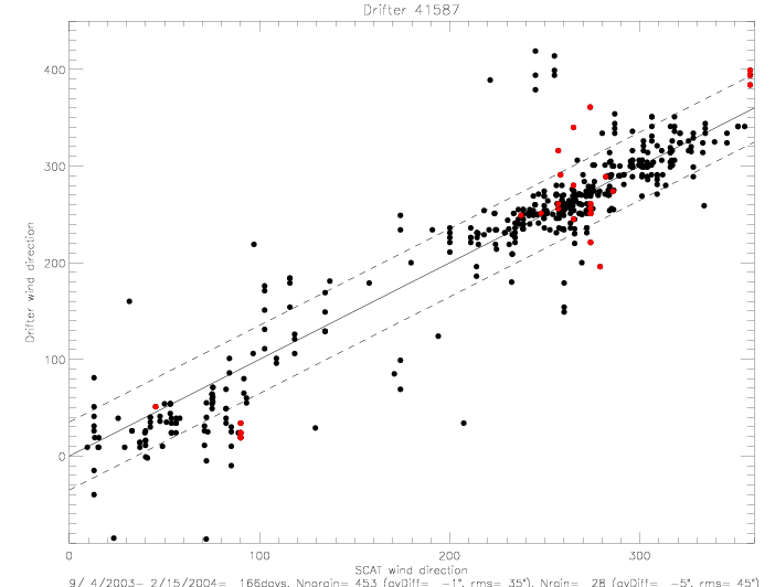 Fig. 6.13 Drifter vs. scatterometer wind directions, for drifters (a) 41582, and (b) 41587.
The collocation statistics for SeaWinds on QSCAT and ADEOS-II are compared in table 6.2: days = number of collocation days,
Ndat = number of collocation pairs, av Dist = average separation distance (km), av Tdiff = average time
difference (scat-drifter, minutes), av Diff = average wind direction difference, rms = rms of wind direction
differences, scat = scatterometer (Q=QSCAT, A = ADEOS-II). SeaWinds on ADEOS-II data are only available until
Oct 24, 2003, so that the ADEOS-II collocation data set is shorter than the QSCAT data set.
Table 6.2: QSCAT and ADEOS-II collocated Wind Directions
| Drifter | days | Ndat | av Dist | av Tdiff | av Diff | rms | scat |
| 41578 | 155 | 563 | 12.1 | -8.6 | -3.4 | 34.3 | Q |
| | 50 | 277 | 16.8 | -7.7 | -3.7 | 39.9 | A |
| 41581 | 153 | 563 | 13.6 | -9.1 | 3.7 | 36.2 | Q |
| | 50 | 247 | 12.9 | -5.3 | 9.0 | 41.0 | A |
| 41582 | 153 | 558 | 13.5 | -9.2 | 0.1 | 43.7 | Q |
| | 50 | 354 | 11.9 | -7.2 | -1.6 | 47.0 | A |
| 41583 | 50 | 253 | 12.9 | -4.5 | 26.2 | 54.3 | Q |
| | 50 | 116 | 15.5 | 4.7 | 27.8 | 40.5 | A |
| 41584 | 162 | 497 | 13.2 | -8.1 | 0.5 | 40.5 | Q |
| | 50 | 302 | 12.4 | -4.1 | -5.8 | 23.3 | A |
| 41585 | 140 | 492 | 12.4 | -7.5 | 1.2 | 29.5 | Q |
| | 50 | 277 | 12.9 | -4.6 | -4.5 | 26.6 | A |
| 41587 | 174 | 559 | 14.6 | -9.8 | 0.0 | 37.0 | Q |
| | 50 | 330 | 12.0 | -6.6 | -1.5 | 28.2 | A |
| 41588 | 148 | 523 | 16.4 | -6.6 | 2.7 | 36.3 | Q |
| | 50 | 312 | 19.2 | -5.5 | -11.4 | 46.7 | A |
A summary of the combined QSCAT and ADEOS-II collocated data is presented in Table 6.3, contrasting no-rain data with
rain-flagged data. Drifter 41583 has a bias in its wind direction measurements, and presents an outlier among this group of drifters.
It transmitted wind direction data for only 50 days, while all other drifters were active for about five months. The average
difference of all other 7 drifters in wind direction of no-rain data is -0.6°, with an rms of 35°. Rain-flagged data have a
bias of -12°(drifter - scat), i.e. drifter wind directions are, on average, 12° counterclockwise from the scatterometer
observations; with an rms of 54°.
Table 6.3: Collocated Wind Direction Differences
| | No Rain | Rain |
| Drifter | av Diff | rms | N | av Diff | rms | N |
| 41578 | -3 | 34 | 421 | -20 | 69 | 44 |
| 41581 | 5 | 35 | 409 | -5 | 49 | 34 |
| 41582 | -1 | 40 | 433 | -8 | 62 | 62 |
| 41583* | 23 | 51 | 207 | 50 | 60 | 17 |
| 41584 | 0 | 32 | 419 | -18 | 67 | 40 |
| 41585 | -1 | 29 | 379 | -4 | 23 | 40 |
| 41587 | -1 | 35 | 453 | -5 | 45 | 28 |
| 41588 | -3 | 38 | 427 | -18 | 42 | 45 |
| | | | | | | |
| av/total* | -1° | 35° | 2941 | -12° | 54° | 293 |
* Note: Drifter 41583 is not included in the averages and totals.
When the drifter wind directions are averaged with a sliding 1-hour window, the comparisons with
collocated scatterometer data do not change very much. Average differences and rms are only slightly
reduced.
Table 6.4: Summary of Collocated 1-hourly Averaged Wind Direction Differences
| | No Rain | Rain |
| Drifter | av Diff | rms | N | av Diff | rms | N |
| av/total* | 0° | 33° | 2941 | -10° | 50° | 293 |
6.b Drifter-to-Drifter Wind Direction Comparisons
Wind direction data of adjacent drifters are compared for 3 pairs of drifters: 41578 & 41585 ,
41584 & 41588 , and 41581 & 41583 . The next three figures show the two time series
in the top panel, the direction differences in the central panel (with the 2-day running average in red,
and the average wind direction difference and rms values printed on the panel), and the distance between
the drifters in the lower panel (in km). Data pairs were only plotted when the distance was less than 50km,
and when the time difference between two drifter measurements was less than 7.5 min. Each drifter measures
wind directions every 15min. Depending on the internal clock of the drifter measuring device, those times
do not fall onto the same real time for all drifters.
Drifters 41581 and 41583 stayed within 50km of each other for the entire time that drifter 41583 was
operational (9/4 - 10/24/2003). Drifter 41583 shows a growing bias with respect to drifter 41581, which is
asumed to be error free. The bias grows from 7.9°(deployment until day 252.4) to 14.3°(days 252.4-258),
and then increases further to 32.4°(days 258-267). After that day the differences are less systematic, and
appear to depend on the prevailing wind direction measured by drifter 41583.
The (drifter-scatterometer) wind direction difference for 41583 is 23° and for 41581 it is 5°.
The (drifter-drifter) difference for (41583-41581) is 19°. This agrees well with the
scatterometer comparions, from which a value of 18° (= 23°-5°) would be expected.
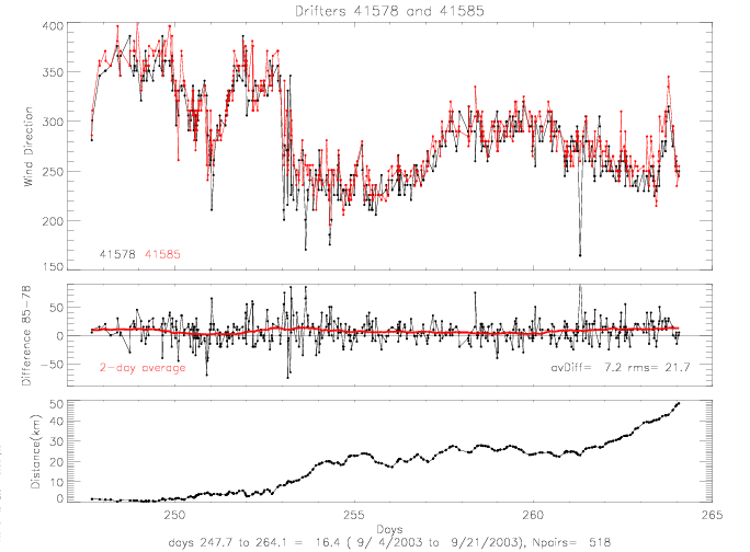
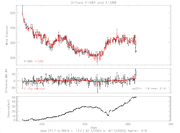 Fig. 6.14 Wind direction differences, for (a) 41585-41578 (16days), and (b)
41588-41584 (13 days).
Fig. 6.14 Wind direction differences, for (a) 41585-41578 (16days), and (b)
41588-41584 (13 days).
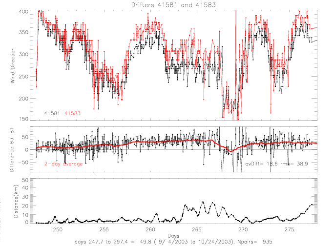
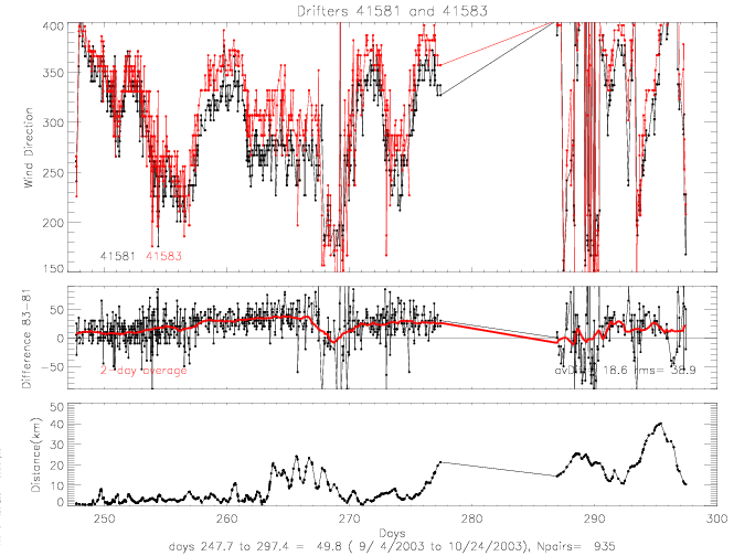 Fig. 6.15 Wind direction differences, 41583-41581, for (a) first 21 days, and (b)
all 50 days.
Fig. 6.15 Wind direction differences, 41583-41581, for (a) first 21 days, and (b)
all 50 days.
7. Drifter Acoustic Noise / Speed
Drifter measured acoustic noise have been processed for all available data. On average, for each drifter
there are about 44 noise observations per day. Similarly to wind direction data, there were about 4 measurements
transmitted to ARGOS about every other hour.
- Sampling Frequency : Acoustic noise is sampled 4 times per hour for 60sec, sampling begins at 12, 27, 42,
and 57min past the hour in drifter time. At every contact with ARGOS, the last 4 samples are transmitted.
- Measurement and Selection / Averaging : The sampling period is 60sec, with 42666 samples/sec for 10000 FFTs,
at 256 points per FFT. Bin averages are created for the following frequency bands: 0-2kHz, 6-10kHz, and 14-20kHz.
The log10 * 20 is taken for each of the final averages for transmission to ARGOS.
- Quality Control at CoRA : The SQL data files have been retrieved from Pacific Gyre, N read ,
and were processed as follows:
- All initial "0,0,0" (0-2,6-10,14-20kHz) values were eliminated ( N 00 ), as were all later 0,0,0 values
( N 0 ), and all records with times that are within 5min of each other and with the same noise values
(N repeat).
- There were also many records within 5min of each other but with different noise data. Those have been
manually edited to eliminate erroneous data spikes (N elim).
A summary of edited data in the first 4 months is presented in Table 7.1.
Table 7.1: Acoustic Noise Quality Control
| Drifter | N read | N 00 | N 0 | N repeat | N elim | N plot |
| 41578 | 10684 | 156 | 20 | 5096 | 31 | 5381 |
| 41581 | 23187 | 176 | 48 | 17494 | 63 | 5405 |
| 41582 | 28952 | 176 | 49 | 22928 | 20 | 5779 |
| 41583 | 2812 | 76 | 143 | 1374 | 6 | 1192 |
| 41584 | 25156 | 204 | 32 | 19344 | 42 | 5534 |
| 41585 | 24572 | 168 | 544 | 18445 | 34 | 5381 |
| 41587 | 23052 | 148 | 64 | 17251 | 67 | 5524 |
| 41588 | 24948 | 144 | 36 | 19237 | 36 | 5479 |
| 41577 | 96 | 68 | 0 | 17 | 3 | 8 |
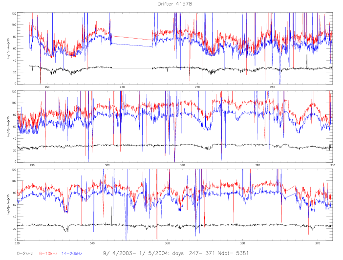
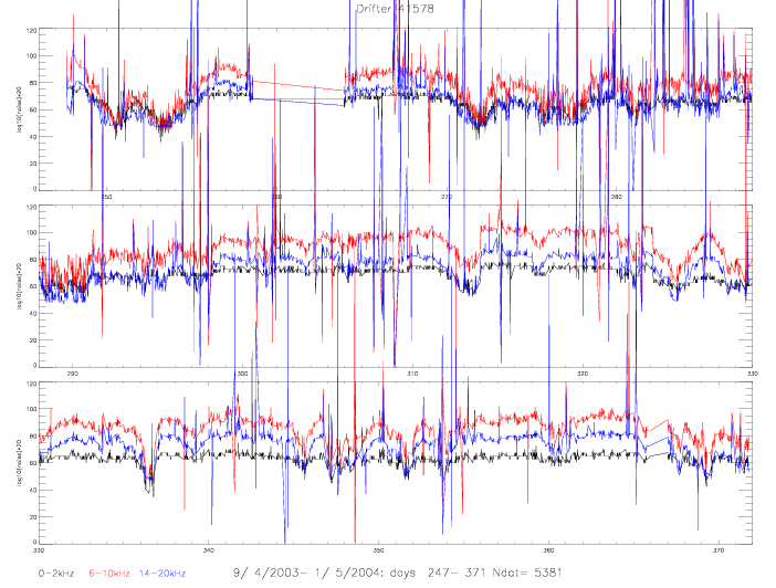 Fig. 7.1 Acoustic Noise from drifter 41578, (a) no scaling, and (b) 0-2kHz scaled by 5/2.
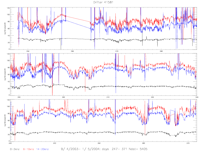
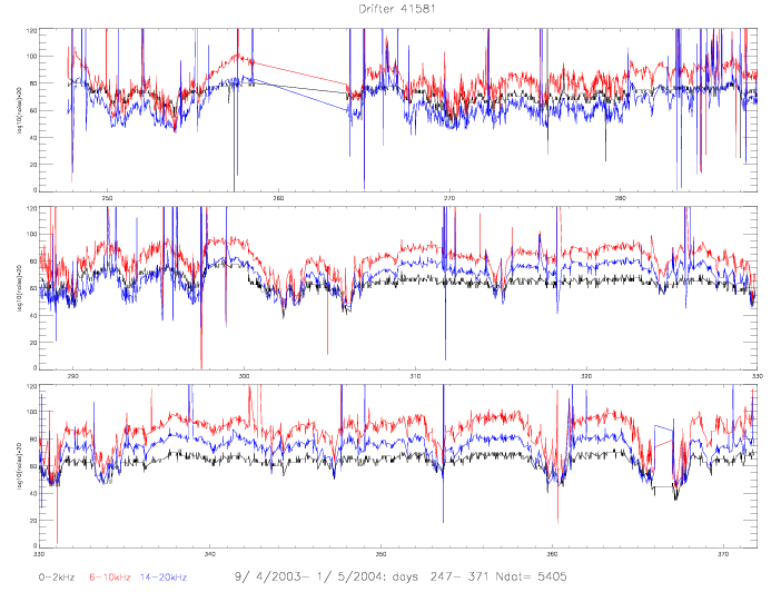 Fig. 7.2 Acoustic Noise from drifter 41581, (a) no scaling, and (b) 0-2kHz scaled by 5/2.
There are still a lot of erroneous (?) spikes in the data. To experiment with additional "spike elimination schemes",
the following steps were taken (and plotted in Fig. 7.3 for (a) drifter 41578 and (b) drifter 41581:
- Plot the 14-20kHz noise for 40 days (days 270-310), to get a detailed look at a subsample of acoustic noise
(panel 1 of Fig. 7.3 a and b). This frequency band seems to be the most noisy of all.
- Eliminate any spikes that are greater than 120 or smaller than 40: 68 records were eliminated in 41578 (panel 2).
- Compute a 3-hr average of the above de-spiked data (plotted in blue in panel no.3).
- Now compute the difference of the de-spiked data and the 3-hr averages. The average difference is
3.3 (diffav), for 41578. Then go through the orginal data, and eliminate all records when the absolute difference of
data - (3hr-average) is less than or equal to 3*diffav: 179 records were eliminated for 41578. This "cleaned-up" data is
plotted in the bottom panel.
- Finally, compute the 3hr average of the cleaned-up data, and overplot (in black) in panel 3. This plot shows
that there is not much gained from continuing with the cleaned-up data and repeating the differencing
one more time to eliminate even more records.
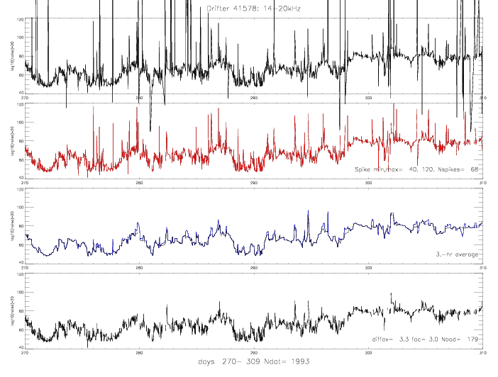
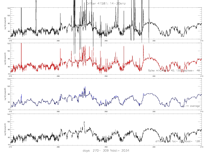 Fig. 7.3 Spike removal scheme, days 270-310 only, for drifters (a) 41578, and (b) 41581.
In figures 7.4 to 7.7, the acoustic noise for all drifters are presented. The frequency band 0-2kHz has been scaled
by a factor of 5/2. Also plotted are the collocated speed data from QSCAT and ADEOS. After 10/24/2003 (day 297) there were no more
ADEOS data available. It appears, that after day 311 the frequency of data from all drifters decreases, so that
collocations are more sparse after this day. In the speed plots, rain-flagged data are marked with open squares,
and no-rain data are marked with filled dots. Also note, that the acoustic noise from drifter 41585 suffers an
apparent malfunction after day 266.5, and before that day, it is much more variable than the data from the other drifters.
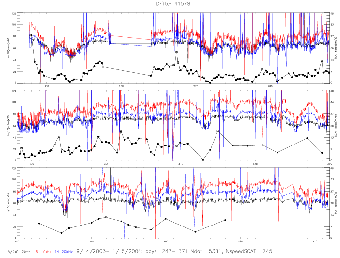
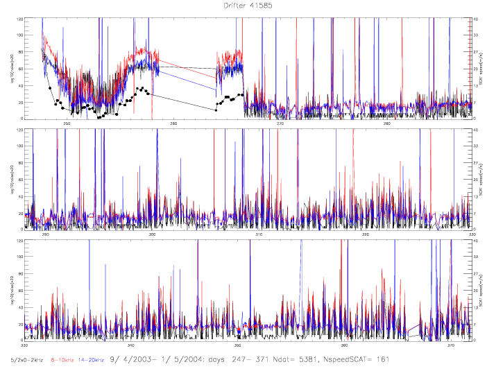 Fig. 7.4 Acoustic Noise and collocated speed, for drifters (a) 41578, and (b) 41585.
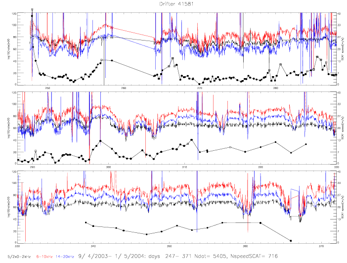
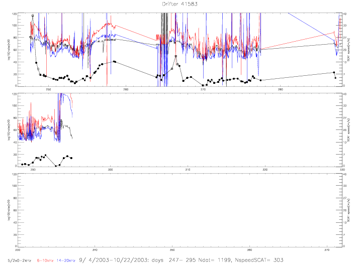 Fig. 7.5 Acoustic Noise and collocated speed, for drifters (a) 41581, and (b) 41583.
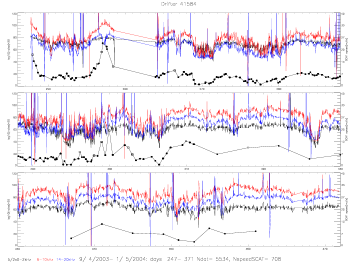
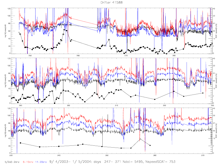 Fig. 7.6 Acoustic Noise and collocated speed, for drifters (a) 41584, and (b) 41588.
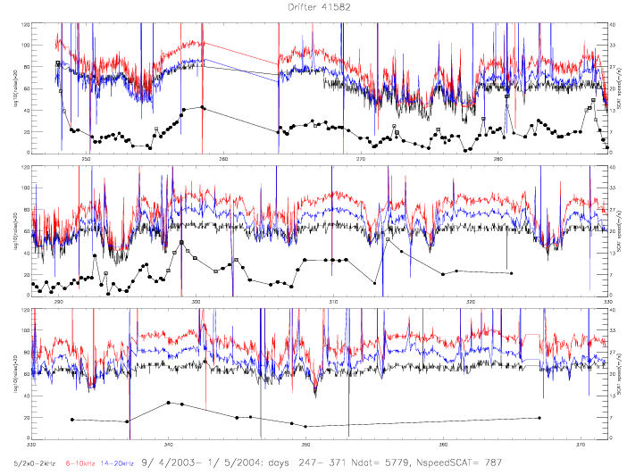
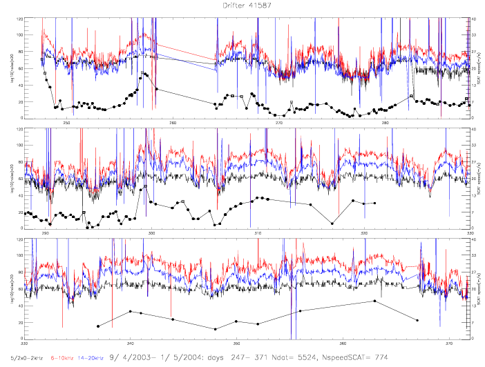 Fig. 7.7 Acoustic Noise and collocated speed, for drifters (a) 41582, and (b) 41587.
8. Acoustic Noise to Speed conversion
Scatter plots of drifter measured acoustic noise vs. nearest scatterometer (QSCAT or ADEOS) measured wind speed are
presented below. For the collocation, a maximum of 100km and 60min separation between drifter and scatterometer
wind vector cells were allowed. On average, however, the average distance was 12-17km and the average time
difference 3-9min.
Fig 8.1 shows the entire range of wind speed (up to 42 m/s), Fig 8.2 shows the range of most data (up to 20 m/s).
All 3 frequencies are plotted (0-2kHz in black, 6-10kHz in red, and 14-20kHz in blue). Note, that the plotted
noise range (on y-axis) does not start with zero. The subtitles under each panel indicate how many plot
points are outside the y-axis range: e.g. for 41581, in the 6-10kHz plot, there are 4 data below and 4 data
above the y-axis range. The big subtitle under all panels indicates how many collocated pairs were found
(e.g. 41581: Ndat = 807), how many speeds fall outside the x-range, and how many scatterometer measurements
were rain-flagged (41581: Nrain = 62). The rain-flagged data are marked with small squares.
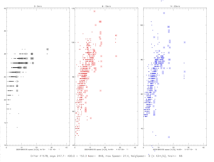
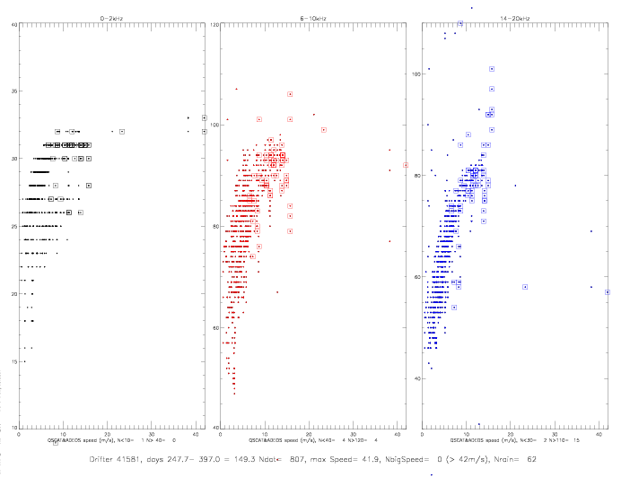 Fig. 8.1 Scatterplots of noise vs. speed (0-42m/s), for drifters (a) 41578, and (b) 41581.
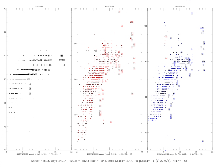
 Fig. 8.2 Scatterplots of noise vs. speed (0-20m/s), for drifters (a) 41578, and (b) 41581.
In order to derive a conversion function between acoustic noise and speed, the following assumptions were made:
- Use linear fit: noise = A + B x speed;
- Eliminate the following data before the first fit:
- eliminate all rain-flagged data,
- eliminate all speeds above 20 m/s,
- eliminate small noise values (<60 for 6-10kHz, <40 for 14-20kHz, none for 0-2kHz);
- Perform a first fit to the data, and compute the rms of (noise-fit) for all data
(this is plotted with dashed black lines);
- Eliminate all data that fall outside the rms limits from the first fit;
- Perform a second fit to the remaining data.
On the following plots, the number of collocated data are listed in all plots (Ndat) ,
the number of data pairs used for the second fit are (Nfit) , the coefficients A and B are
listed (Cof) , and all rain-flagged data are marked with open squares and counted as
(Nrain) . Also plotted are the rms of the second fit (with red dashed lines), and the resulting
Sp rms are listed. "Sp rms" is a measure of the scatter of the second fit in speed units (m/s);
it is the horizontal distance between the two red dashed lines. Note, that
the accuray of scatterometer measured wind speed is estimated to be 2 m/s rms.
Several drifters have bad acoustic noise data towards the end of the record: drifter 41578 goes bad
on day 400, drifter 41585 on day day 266.5 (see Fig. 7.4b), and drifter 41587 at day 376.
Those periods are excluded from the collocation and conversion to speed.
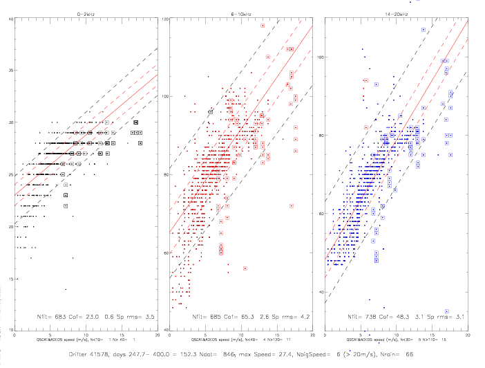
 Fig. 8.3 Linear fit, for drifters (a) 41578, and (b) 41585.
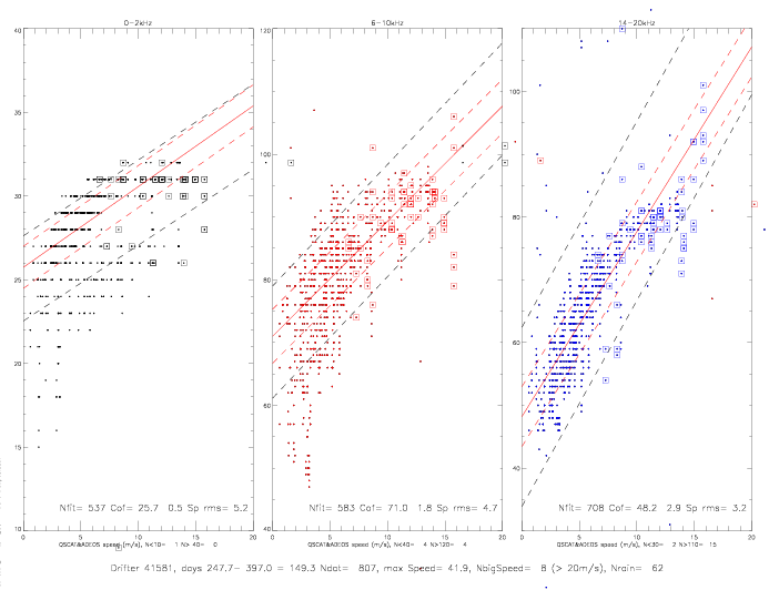
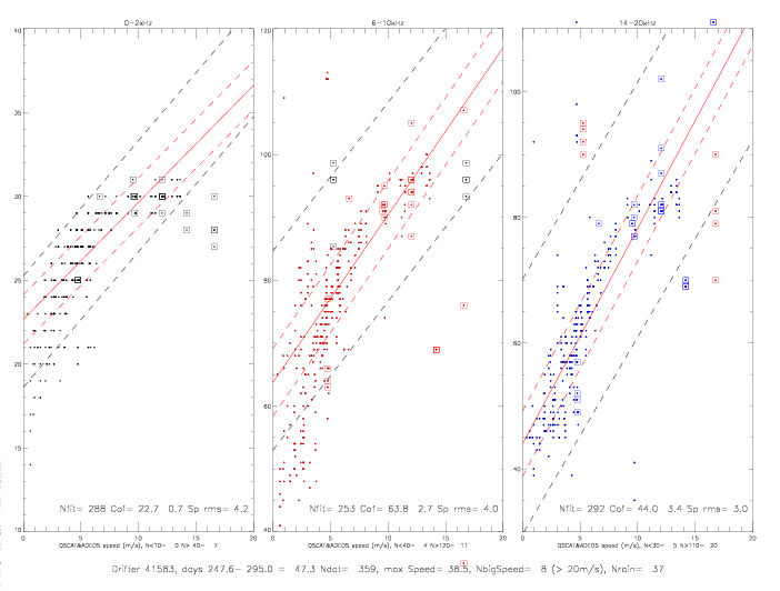 Fig. 8.4 Linear fit, for drifters (a) 41581, and (b) 41583.
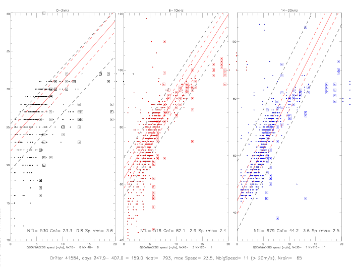
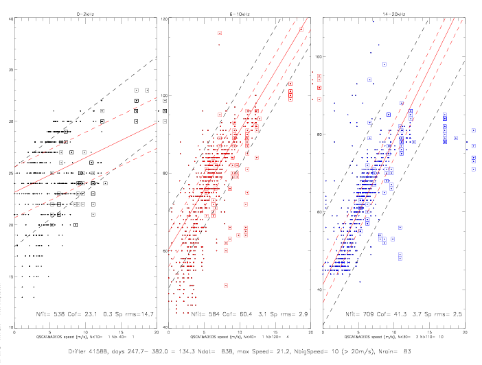 Fig. 8.5 Linear fit, for drifters (a) 41584, and (b) 41588.
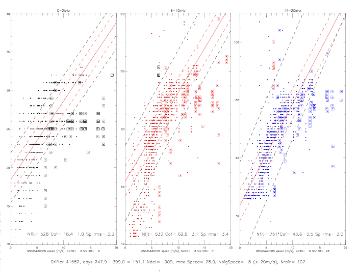
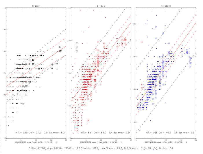 Fig. 8.6 Linear fit, for drifters (a) 41582, and (b) 41587.
The conversion coefficients are summarized in the table below. Also listed are the number of days in the
data sets, the number of data for the linear fit, Nfit, and the resulting rms differences between
derived speeds and collocated SCAT speeds. The 0-2kHz frequency turns out to be the most unreliable,
and in some drifters it drops to lower levels half-way through the data record (as can be seen in figures 7.4-7.7).
Therefore, the 0-2kHz derived speed estimates are not used.
Table 8.1: Noise-to-Speed conversion: Noise = A + B x Speed
| | 6 - 10 kHz | 14 - 20 kHz |
| Drifter | Days | Nfit | A | B | rms | Nfit | A | B | rms |
| | | | | | |
| | | |
| *41583 | 47 | 253 | 64 | 2.7 | 4.0 |
292 | 44 | 3.4 | 3.0 |
| *41585 | 19 | 122 | 49 | 2.8 | 3.0 |
135 | 29 | 3.5 | 2.9 |
| | | | | | |
| | | |
| 41578 | 152 | 685 | 65 | 2.6 | 4.2 |
738 | 48 | 3.1 | 3.1 |
| 41581 | 149 | 583 | 71 | 1.8 | 4.7 |
708 | 48 | 2.9 | 3.2 |
| 41582 | 151 | 633 | 62 | 3.1 | 3.4 |
751 | 44 | 3.5 | 3.0 |
| 41584 | 159 | 516 | 62 | 2.9 | 2.4 |
679 | 44 | 3.6 | 2.5 |
| 41587 | 127 | 651 | 63 | 2.4 | 3.9 |
766 | 49 | 2.6 | 3.9 |
| 41588 | 134 | 584 | 60 | 3.1 | 2.9 |
709 | 41 | 3.7 | 2.5 |
| | | | | | |
| | | |
| *average | 151 | 609 | 64 | 2.7 |
3.6 | 725 | 46 | 3.2 |
3.0 |
* Note: Drifters 41583 and 41585 are not included in averages.
With the above derived conversion coefficients the entire acoustic noise data were converted to
speed, for both 6-10kHz (red lines) and 14-20kHz (blue lines) derived speeds. Presented are the speed estimates
from all drifters (no spikes removed), for the first 4 months.
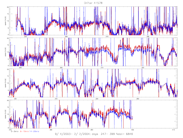
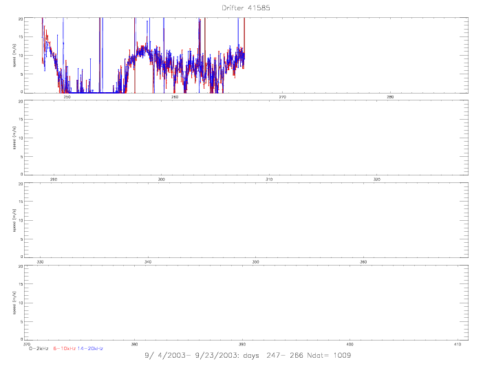 Fig. 8.7 Speed estimates, for drifters (a) 41578, and (b) 41585.
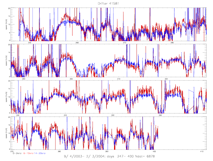
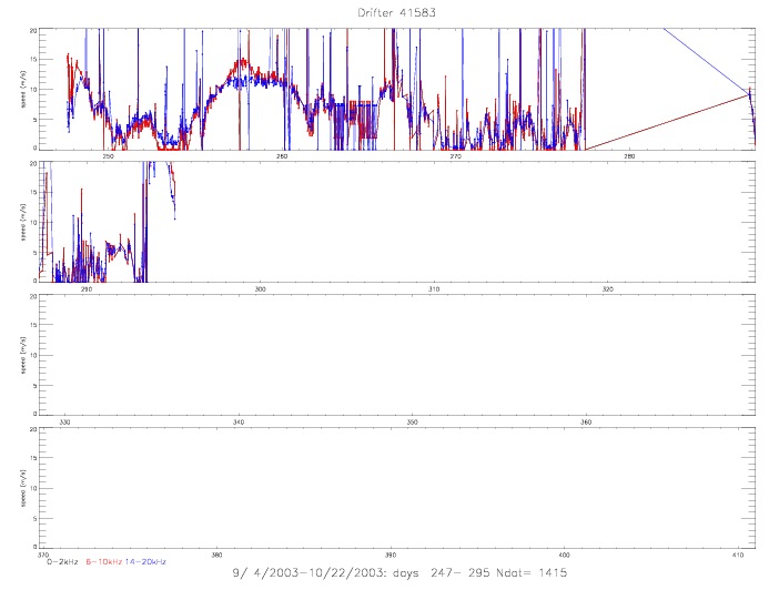 Fig. 8.8 Speed estimates, for drifters (a) 41581, and (b) 41583.
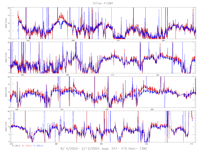
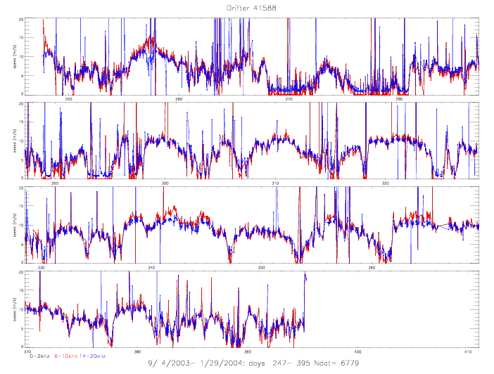 Fig. 8.9 Speed estimates, for drifters (a) 41584, and (b) 41588.
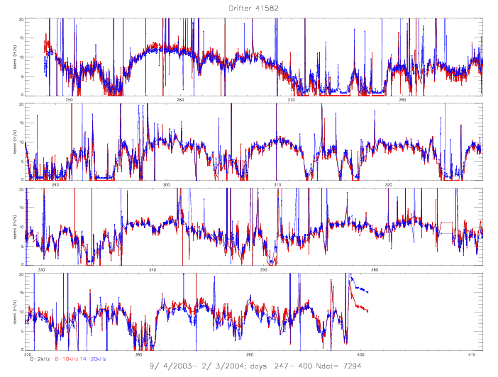
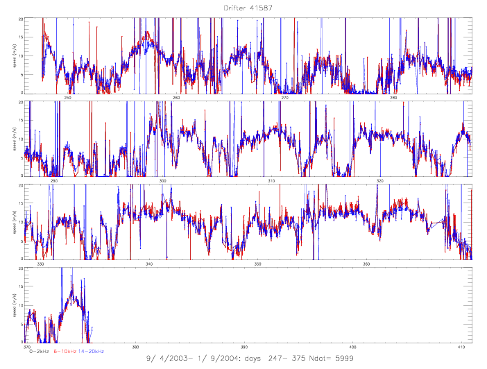 Fig. 8.10 Speed estimates, for drifters (a) 41582, and (b) 41587.
De-spiking of Speed Estimates
To remove, as much as possible, the spikes in the speed record, the following procedure was used:
- Compute a smoothed record with a running average of 3-hr.
- Compute the average difference between the 3-hr smoothed record and the original data (avdiff).
- Then, eliminate all spikes whenever the absolute difference > 3*avdiff.
- Repeat the above steps three times.
- Finally, by visual inspection remove remainding spikes (usually ca. 30 spikes).
On average, about 1400-2100 spikes were removed for each frequency band. The resulting speed records
are plotted below, for the 6-10kHz (red) and 14-20kHz (blue) derived speeds.
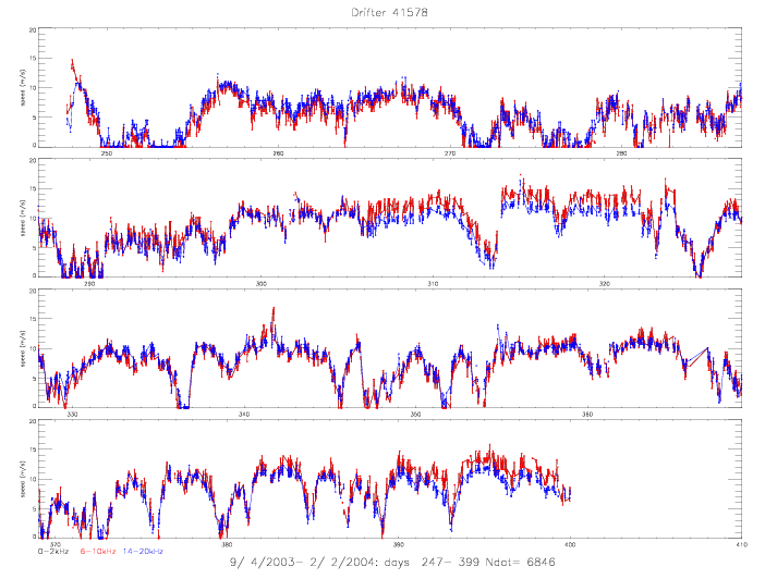
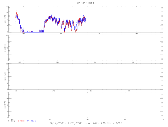 Fig. 8.11 De-spiked speed estimates, for drifters (a) 41578, and (b) 41585.
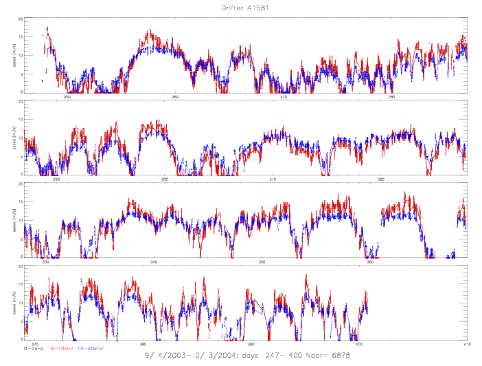
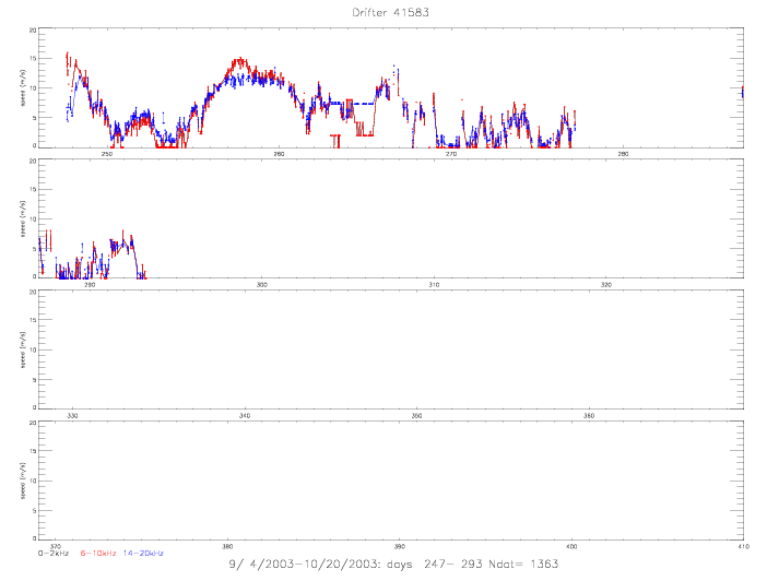 Fig. 8.12 De-spiked speed estimates, for drifters (a) 41581, and (b) 41583.
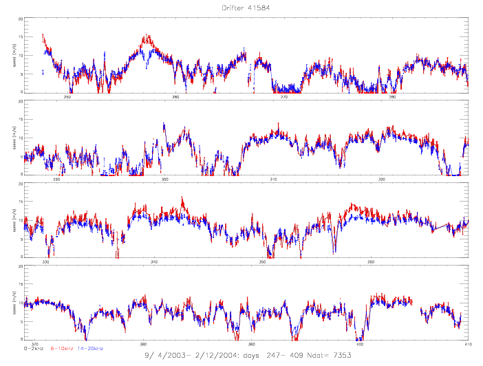
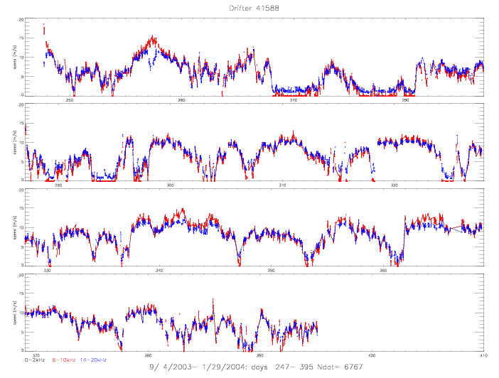 Fig. 8.13 De-spiked speed estimates, for drifters (a) 41584, and (b) 41588.
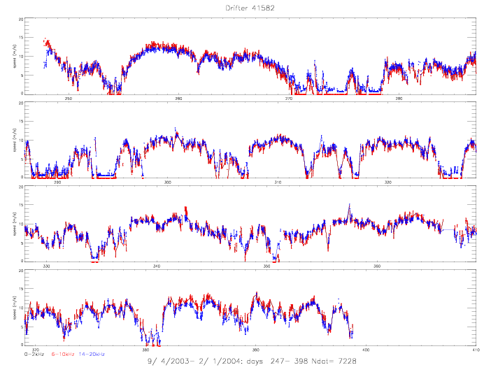
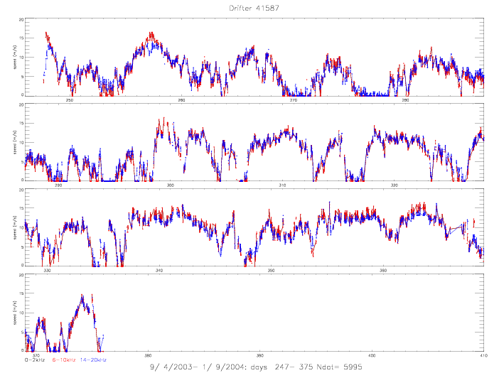 Fig. 8.14 De-spiked speed estimates, for drifters (a) 41582, and (b) 41587.
In order to examine the differences in speed between the two frequency bands, 6-10kHz and 14-20kHz,
1-hourly averages were computed. Also plotted below are the collocated scatterometer speeds:
solid dots for non-rain and open squares for rain-flagged data.
When both scatterometers were operating there were 3-4 collocations per day (days 247-297, 9/4/-10/24/2003).
After ADEOS-II stopped transmitting data there were only 1-2 collocations per day (days 297-310,
10/24-11/6/2203). After day 310, however, the collocations dropped to only one for every 3 or 4 days, because
almost no drifter data were transmitted between 3-7am and 2-6pm local time (see Fig. 1.0).
The QSCAT overflights happened usually around 5am and 5pm. Note the relatively high SCAT wind speeds
at the beginning of the record (day 247), which are associated with hurricane Fabian.
As usual, drifter figures are paired so that nearby drifters are shown netx to each other:
41578 & 41585, 41581 % 41585, 41584 & 41588, and 41582 and 41587 (which are not as close to each other
as the other pairs).
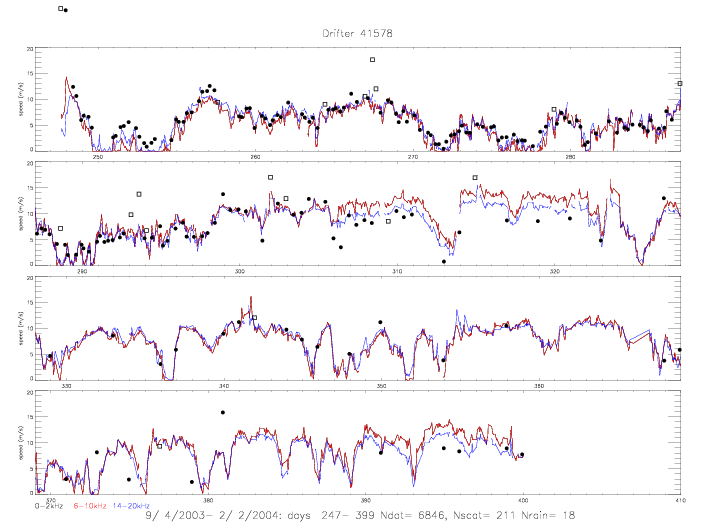
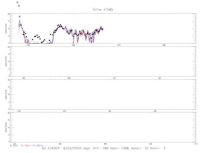 Fig. 8.15 1-hourly speed averages and collocated SCAT data, for drifters (a) 41578, and (b) 41585.
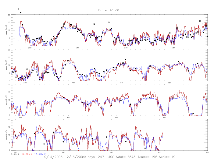
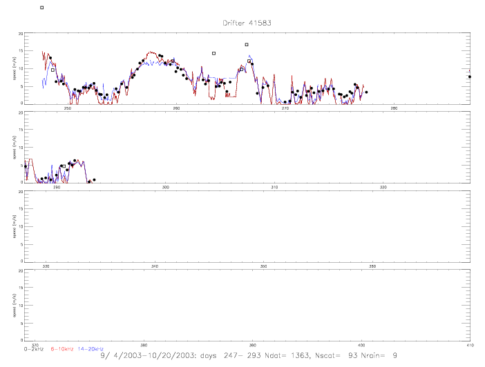 Fig. 8.16 1-hourly speed averages and collocated SCAT data, for drifters (a) 41581, and (b) 41583.
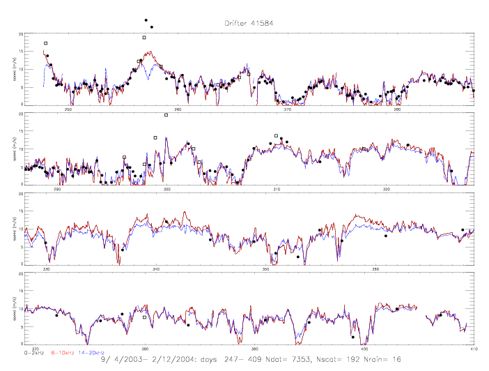
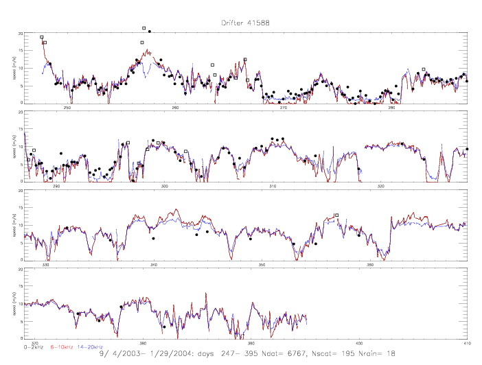 Fig. 8.17 1-hourly speed averages and collocated SCAT data, for drifters (a) 41584, and (b) 41588.
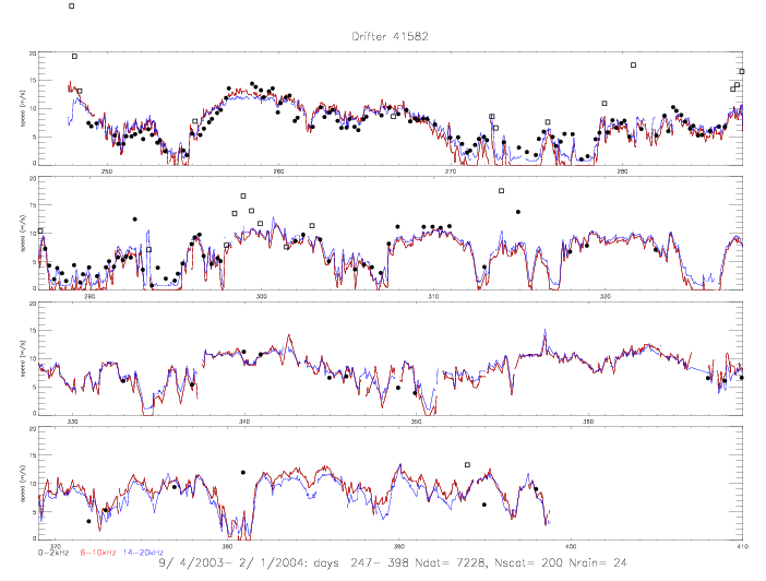
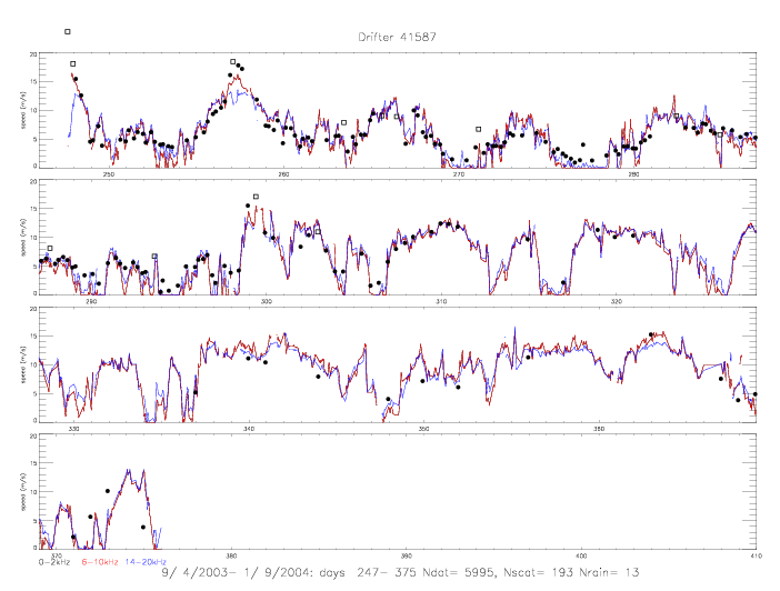 Fig. 8.18 1-hourly speed averages and collocated SCAT data, for drifters (a) 41582, and (b) 41587.
None of the drifters can capture the very high winds from nearby hurricanes Fabian (day 247) and Isabel (day 257),
when scatterometer speeds exceed 20m/s. There are instances when the 14-20kHz derived speeds drop as the 6-10kHZ
rise: in particular when Isabel passes around day 257 - see drifters 41581 & 41585, and 41584 & 41588.
Each drifter exhibits time periods when the two frequency derived speeds differ from each other by an almost
constant offset for long periods of time. Then there are also time periods when both speeds fall right on top of each other.
For example in drifter 41581, the two speed estimates track each other pretty well for days 259-273; for next 27 days
(273-300) the 14-20kHz speeds are lower than the 6-10kHz speeds by about 2-3 m/s, with collocations favoring the lower
14-20kHz estimates; for the time period 300-319 the 14-20Hz speeds are larger than the 6-10kHz estimates -
again, the collocations seem to agree more with the 14-20kHz estimates. There are may instances, however, when
the 6-10kHz speed estimates agree better with the collocated SCAT speeds: e.g. see drifter 41588 during days
310-312.
The accuray of the two freqency derived speed estimates is investigated for different speed ranges.
In the figure below, all collocations are shown for all drifters. The speed differences (Drifter-SCAT) are
plotted versus SCAT speeds. Not included are rain-flagged data and drifter speeds less than 0.2m/s.
Averages and standard deviations are computed in 2m/s bins, and shown as well (plotted with a slight
offset from the bin center, so that the two frequency estimates can be differentiated from each other). The number
of data in each 2m/s bin are printed on the bottom of the figure.
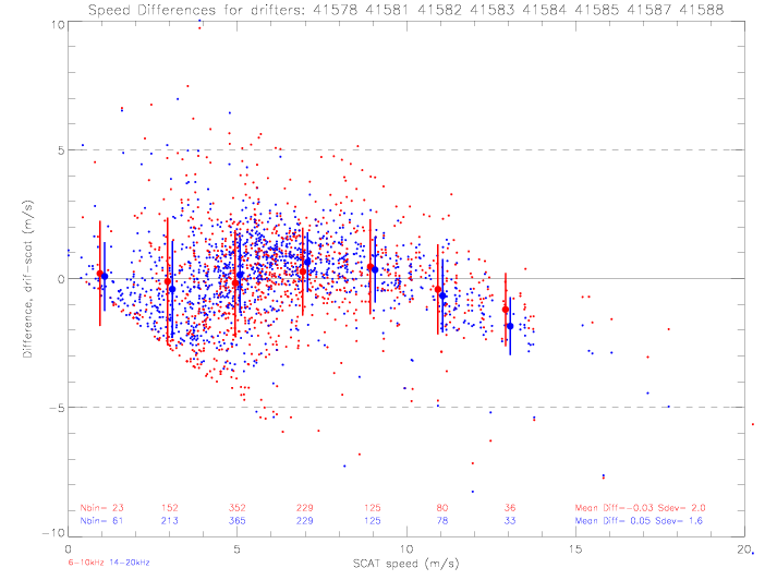 Fig. 8.19 Speed differences (drifter-SCAT) vs. SCAT speeds, including 2m/s bin averages and standard deviations.
There is quite a scatter around the 0m/s difference line. Over most of the speed range (0-12m/s), the bin averages
are within 0.5m/s of SCAT measured speeds. The estimates from the two frequencies behave very similar.
At low speeds (<5m/s), the estimates tend to be too small, between 5 and 10m/s the estimates are slightly too
large, and they increasingly underestimate the wind speed above 10m/s.
The standard deviations range between 1.1 and 2.5m/s. The 14-20kHz speed estimates have lower standard deviations
than the 6-10kHz derived speeds, by about 0.5m/s.
Over the speed range of 0.2-15m/s, the overall mean difference for 6-10kHz is -0.03m/s (St.Dev.= 2.0m/s, N = 1,011);
the mean for 14-20kHz is 0.05m/s (St.Dev.= 1.6m/s, N = 1,118).
A scatterplot of the two derived speed estimates is presented below. For all speeds (>0), the average difference
between the 14-20kHz and 6-10kHz speed estimates is 0.16m/s (St.Dev. = 1.4m/s, N=1,124).
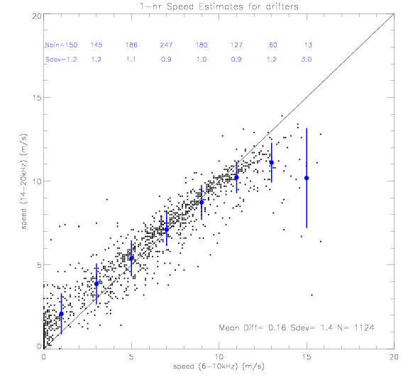 Fig. 8.20 Scatterplot of 14-20kHz dervived speeds vs. 6-10kHz speeds.
1-hourly speed estimates for the first 15 days (during hurricanes Fabian and Isabel)
In order to concentrate on the time interval when the drifters were closest to Fabian (9/4 = day 247)
and Isabel (9/14 = day 257), the plots below show the first 15 days, i.e. days 247-262. Both the 6-10kHz
and 14-20kHz derived speed estimates are plotted, together with the collocated speeds from QSCAT and
ADEOS-II. Rain-flagged data are marked with open squares, no-rain data are marked with solid
dots. Assuming that the scatterometer speeds are "true", it is remarkable how well the acoustic
noise picks up short-term fluctuations in wind speed: e.g. drifter 41587 during days 250.5 to 252.5.
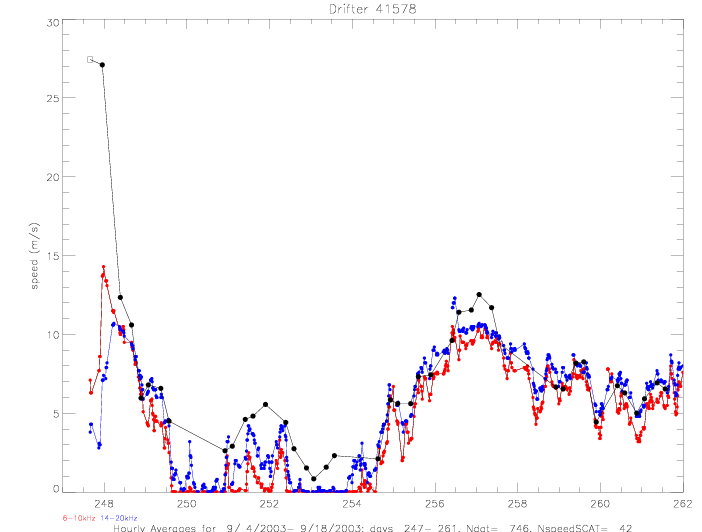
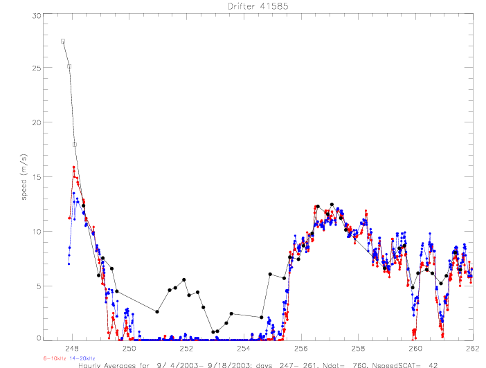 Fig. 8.21 1-hourly averaged speed estimates, for drifters (a) 41578, and (b) 41585.
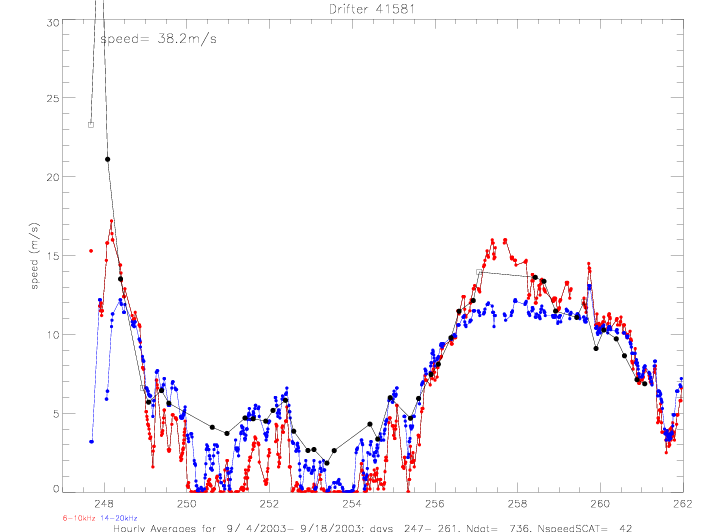
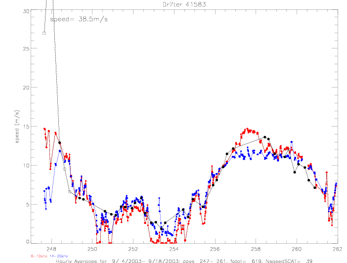 Fig. 8.22 1-hourly averaged speed estimates, for drifters (a) 41581, and (b) 41583.
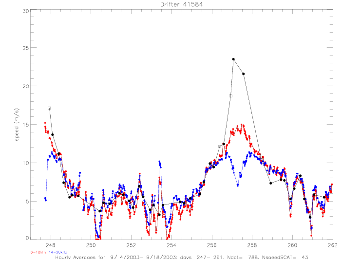
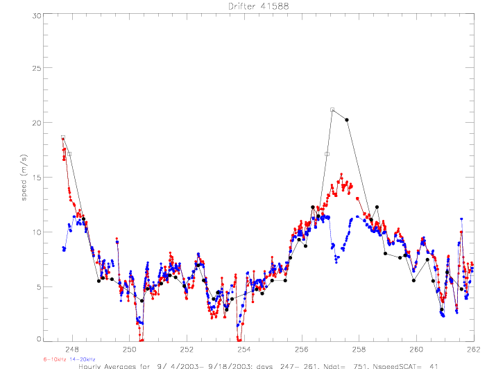 Fig. 8.23 1-hourly averaged speed estimates, for drifters (a) 41584, and (b) 41588.
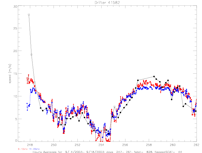
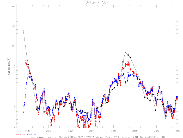 Fig. 8.24 1-hourly averaged speed estimates, for drifters (a) 41582, and (b) 41587.
9. Figures and text for Poster at AGU Ocean Sciences meeting (Portland, January 26-29, 2004)
Drifter Observations in Hurricane Fabian
Preliminary Report
Peter Niiler, Willliam Scuba (Scripps Institution of Oceanography), and
Jan Morzel (Colorado Research Associates, NWRA)
The pdf file of the finished poster can be viewed and downloaded from
here .
The text and figures are listed below. Minor changes were made to figure 1, which now includes the specs
for the Minimet instruments, and to the caption of figure 5 (20-30N, 60-70W).
Minimet Drifter and Deployment Tests (1. column)
Observations of the response of the ocean to storms can be done with ARGOS tracked drifters. Minimet drifters
are configured to measure wind speed with a WOTAN, wind direction, SST, sea level air pressure, and Lagrangian
displacement at 15m depth (Milliff et al., 2003). The 53rd USAF Air National Guard "Hurricane Hunter"
squadron was trained to deploy parachute rigged boxes, each containing two Minimets, from C-130-J aircraft. The
deployment of containers was successful both at sea and over land. In August, 2003, the USAF has approved the
deployment container system of Minimets as 'operational' from C-130-J aircraft.
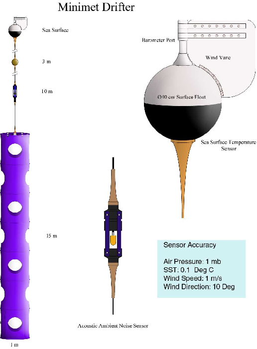
Figure 1. Schematic of Minimet Drifters
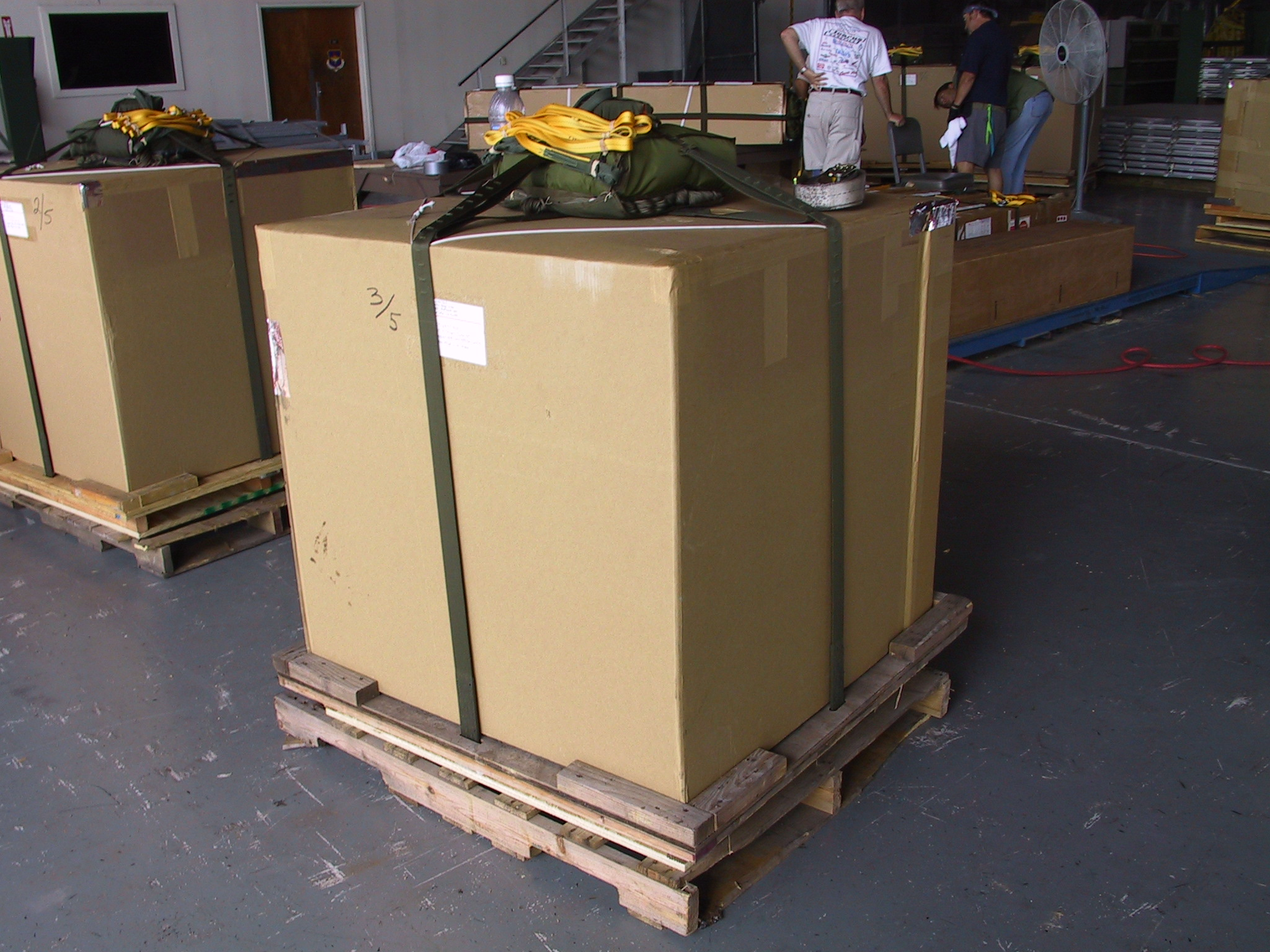
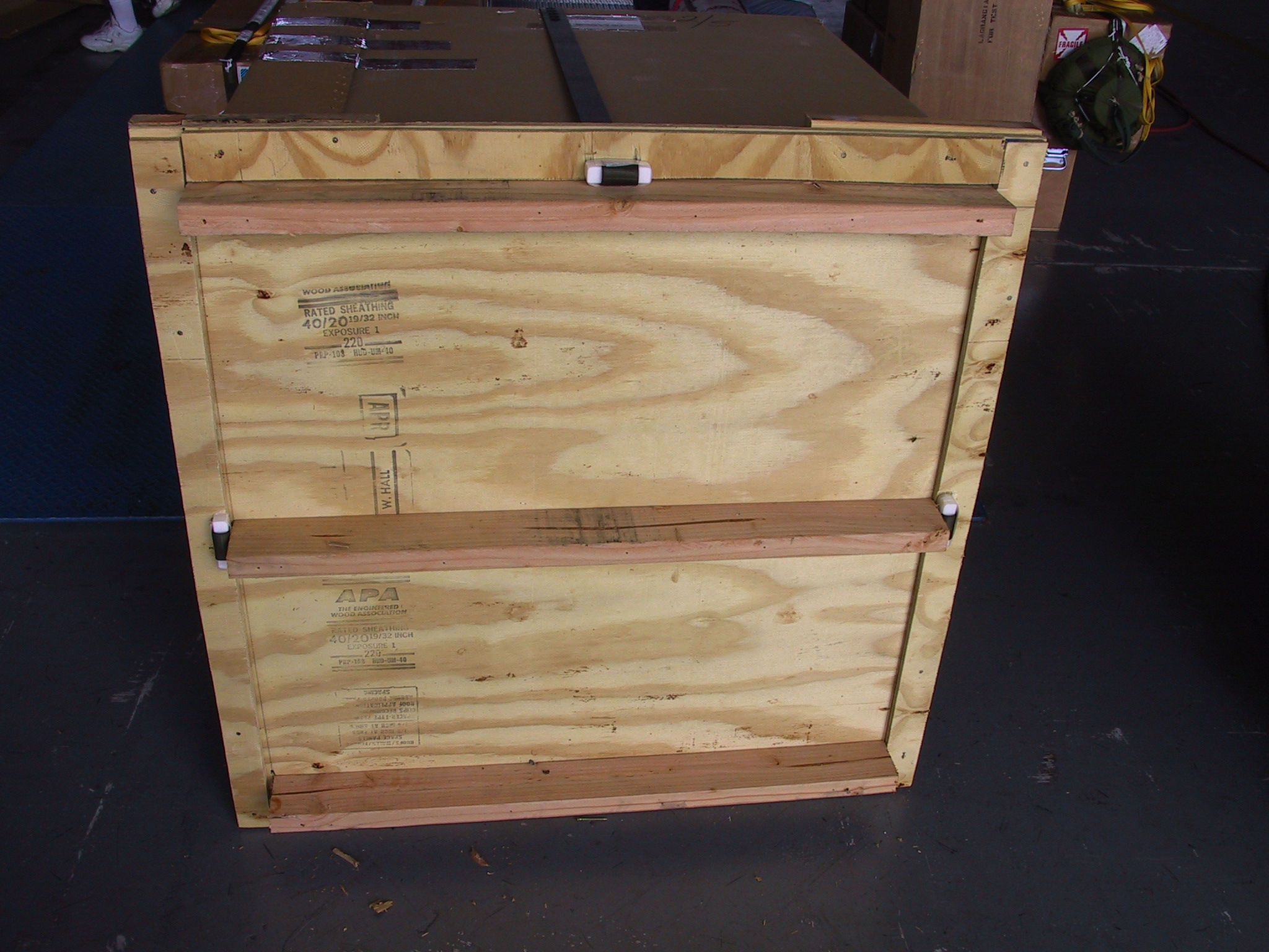
Figure 2.a and b
Deployment containers and salt block release: each box contains two Minimet drifters and is strapped to an
air deployment pallet. The shipping pallet underneath is removed before deployment. The picture on the right
shows the underside of the deployment pallet with the bottom plywood removed. There are salt blocks holding the
parachute rigging in place.
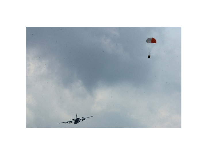
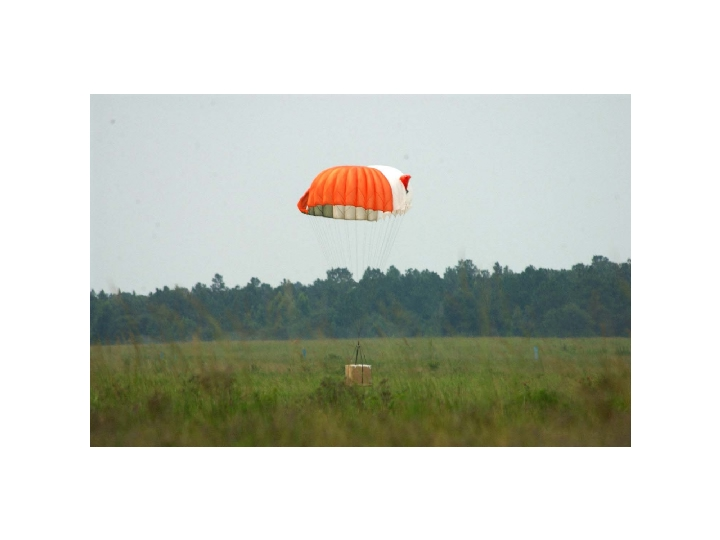
Figure 3.a and b
C-130-J aircraft and deployment package parachuting to the ground during over land testing; and
deployment package landing in a field during testing.
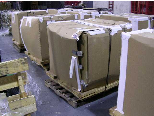
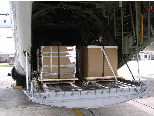
Figure 4.a and b
Air deployment package damaged during shipping; and repaired air deployment packages being loaded on a C-130-J
aircraft.
Drifter Deployment in Fabian (2.column)
On September 4, 2003, 16 Minimets in 8 containers were parachuted from a Hurricane Hunter C-130-J in front
of hurricane Fabian, which had 120 knot sustained winds. In 36 hours following the deployments, Fabian
passed over the Minimet array, 8 of which survived and continued to produce data for 5 months afterwards.
A research vessel picked up one Minimet after 21 days at sea - its mechanical configuration was intact and
showed no wear or tear due to Fabian passage.
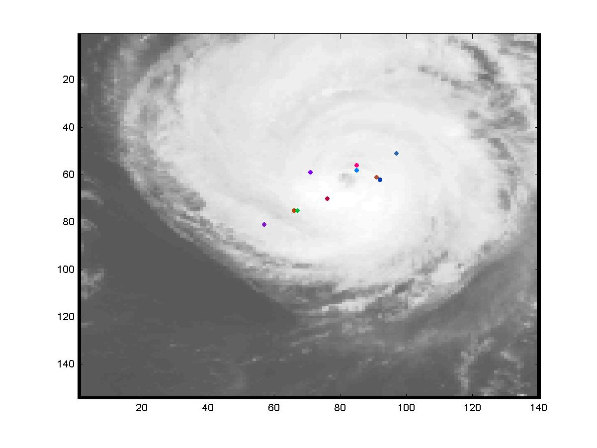
Figure 5. Location of drifters at their closest position to the center of hurricane Fabian (20-30N,60-70W).
Figure 6.
Hurricane Fabian depicted by scatterometer derived wind vectors during 32 hours, and near-simultaneous drifter
wind directions. The time differences (drifter-scat) are indicated below the figures. Rain-flagged scatterometer
data are plotted in red (wind speeds ${<}$ 15m/s) and green (wind speeds ${\ge}$ 15m/s). The blue crosses mark
the scatterometer implied hurricane centers. The red crosses depict the NOAA centers, interpolated in time to
scatterometer overflight time.
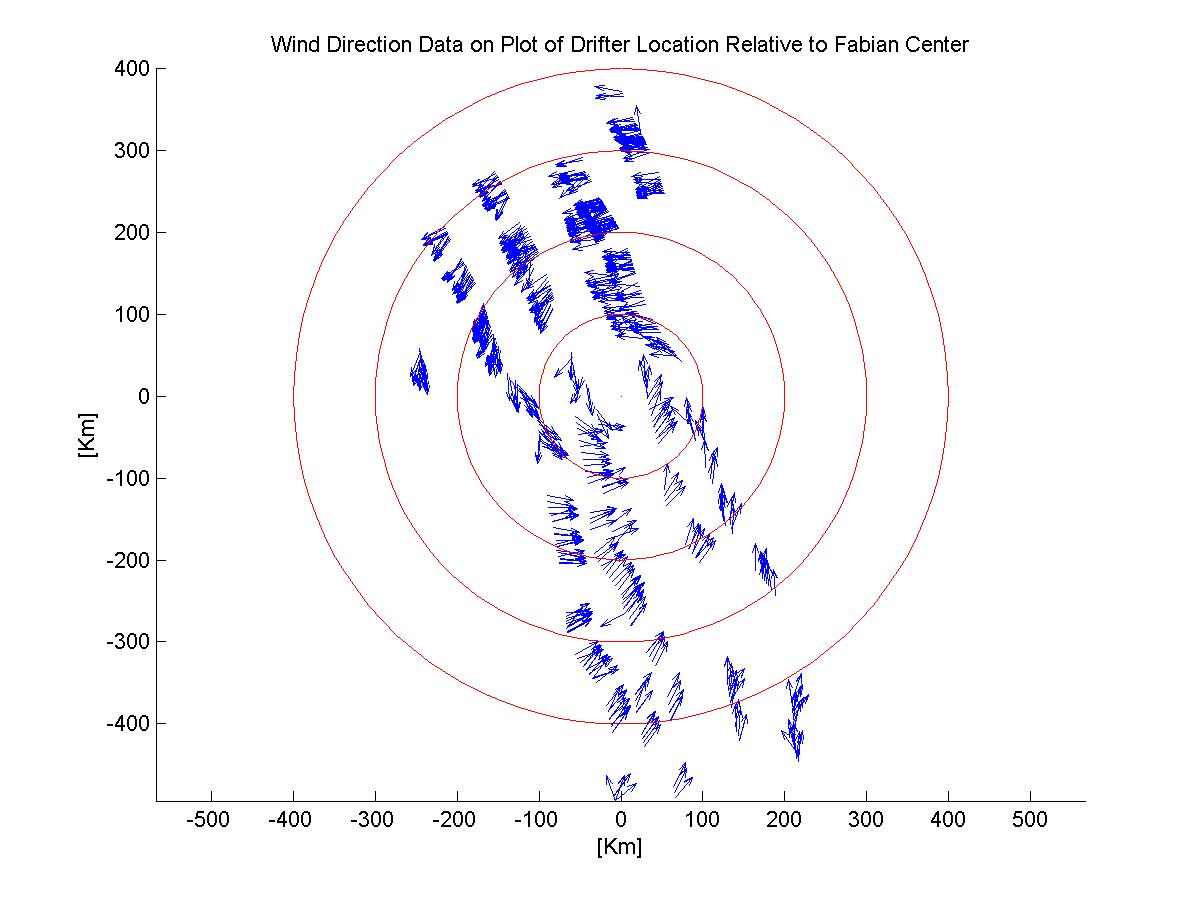
Figure 7. Drifter observed wind directions during the passage of hurricane Fabian.
Time Series of Observations (3. column)
Time series of measurements from drifters 41581 and 41587 show that the 'center' of Fabian passed over the Minimet
array. The 'center' of Isabel, a class 5 hurricane, also came near the array. The pressure near Fabian
'center' dropped from 1018 mb to 942 mb, which compares well with airplane dropsond observations of 939-946mb on
September 4. The Minimet direction of the wind relative to Fabian 'center' shows a change of the direction
of the radial component of 'inflow' at a radius of 320 km and another change at a radius of 80 km. SST cooled
in the center of Fabian by 2°C SST, establishing a 'cold wake'. SST recovered within six days inside the
'wake' to the surrounding night-time temperature of 27.7°C.
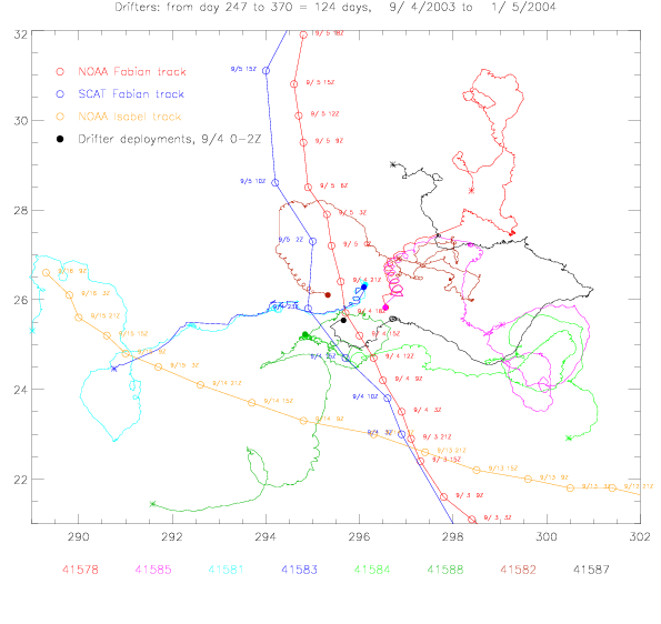
Figure 8.
Drifter tracks and locations of hurricane Fabian and Isabel.
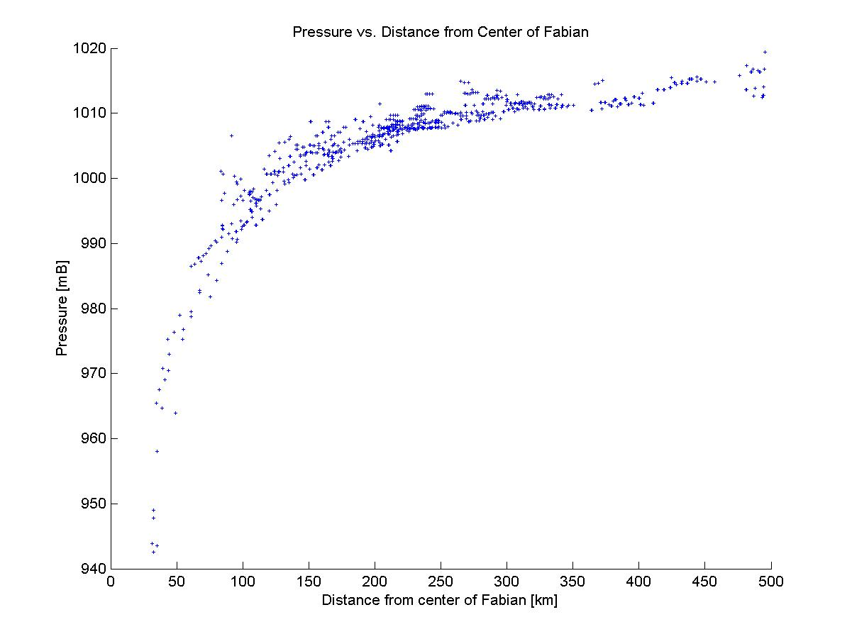
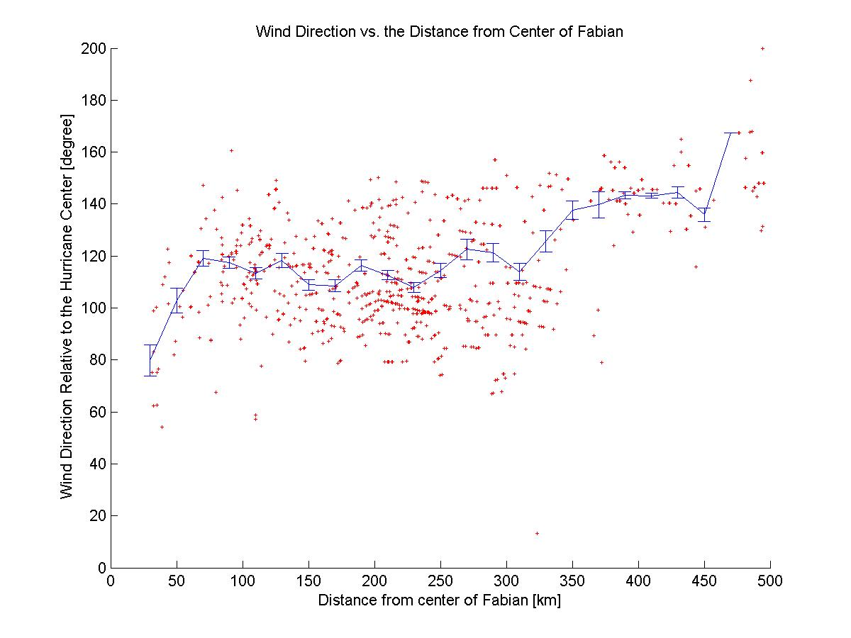
Figure 10.a and b
Sea level air pressure and wind direction relative to the center of hurricane Fabian, during the first 48
hours after deployment. An angle of 0° corresponds to a wind blowing directly away from the
hurricane center. Angles increase as the wind rotates counterclockwise. Angles above 90° indicate
wind blowing towards the center.
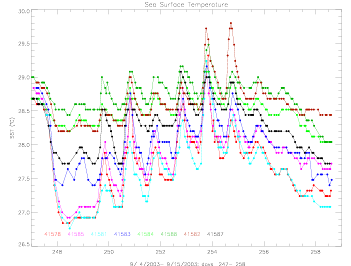
Figure 11.
Sea Surface Temperature from all drifters during the first 12 days after deployment.
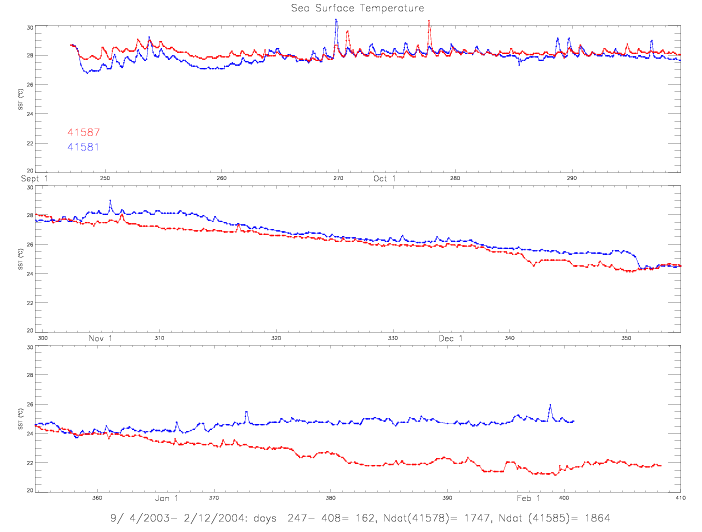
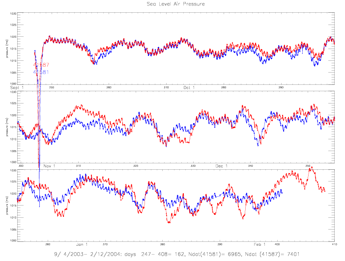
Figure 12.a and b
Sea surface temperature and sea level air pressure from drifters 41581 and 41587.
Comparison with Scatterometer Winds (4. column)
The 25 km scale wind speed and wind direction from SeaWinds on QSCAT and ADEOS-II scatterometer swath data
were collocated with the drifter observations. On average, the observations are within 12-17km and 3-9min.
The ${\log}_{10}$ of ambient noise from the 6-10 kHz band from Minimets showed a linear relationship to wind
speed over 2m/s to 17m/s, at which point saturation of the sound spectrum became apparent. The wind
direction compared well without bias, except for those scatterometer cells that were rain-flagged.
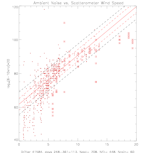
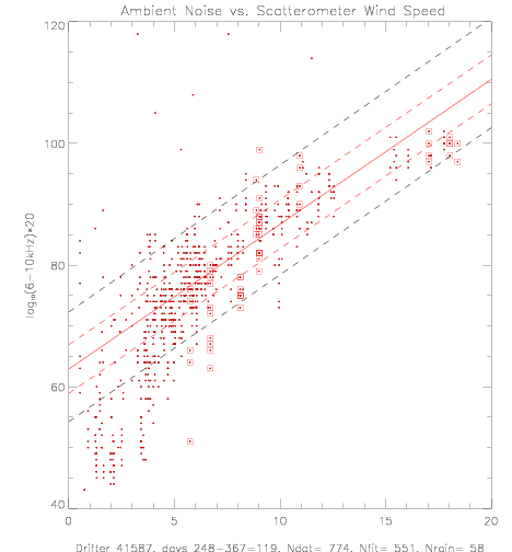
Figure 13.
Ambient noise vs. collocated scatterometer speed (for 6-10kHz band, drifters 41584 and 41587).
All rain-flagged speeds and all noise below 60 on the y-axis were excluded from the fit. An initial fit was
performd, for which the rms is plotted with black dashed lines. All data outside of ${\pm}1$ rms were
excluded from the final fit (Nfit), which resulted in the red line and its rms (red dashed lines).
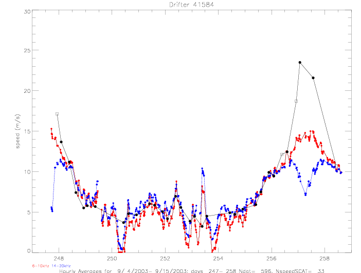
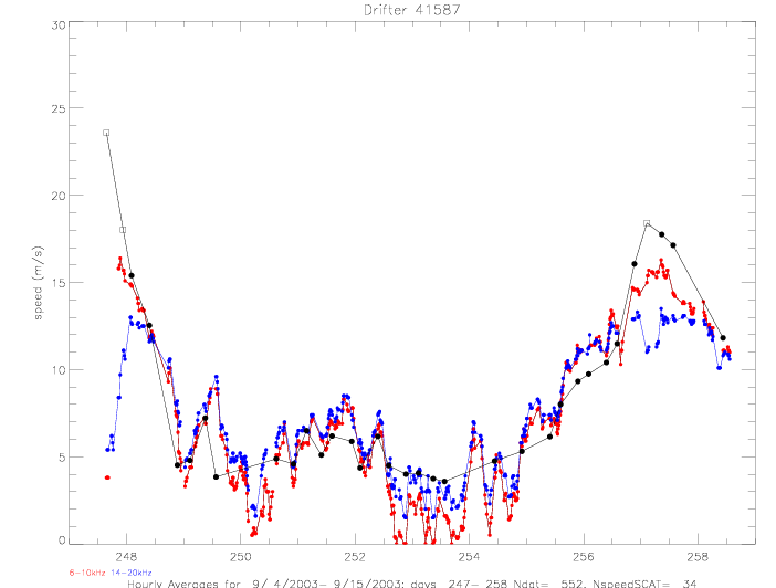
Figure 14.
Drifter speed (converted from ambient noise) for the first 12 days after deployment.
Hourly averages are plotted for drifters 41584 and 41587.
Collocated scatterometer measurements are depicted as solid dots (not rain-flagged) and
open squares (rain-flagged).
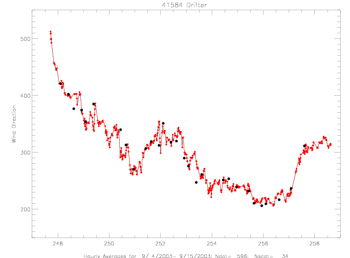
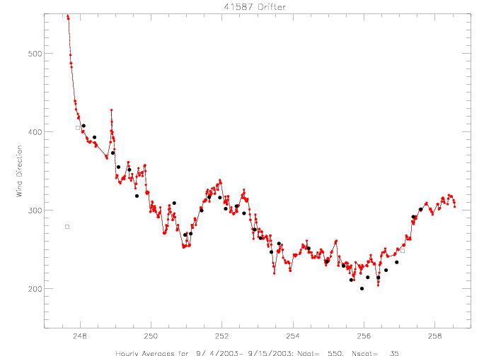
Figure 15. As above, but for wind direction.
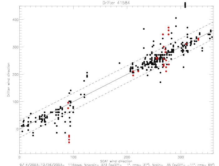
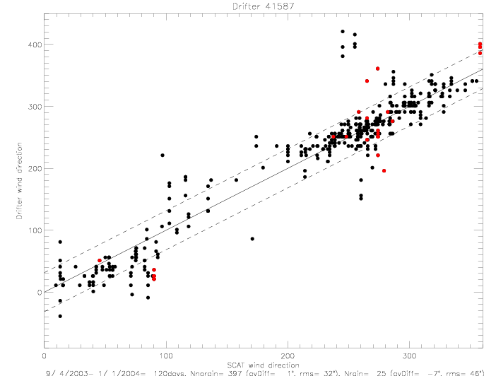
Figure 16.
Wind direction scatterplot of drifter and scatterometer observations (drifters 41584 and 41587).
The 1:1 line is plotted and the rms of no-rain flagged data is indicated by dashed lines.
When all drifter data are combined, the average difference is 0.1°, with an rms of 35° for
a total of 2588 no-rain flagged data. The rain-flagged data (N=274) has a bias of -9° (drifter-scat),
with an rms of 53°.
References
Milliff, R.F., P.P. Niiler, J. Morzel, A.E. Sybrandy, D. Nychka, and W.G. Large, 2003:
Mesoscale Correlation Length Scales from NSCAT and Minimet Surface Wind Retrievals in the Labrador Sea.
J. Atmos. Oceanic Technol. , 20 , 513-533.
last modified on February 16, 2005
Go
Back
)
)
)
)
)
)
)
)
)
)
)
)
)
)
)
)
)
)
)
)
)
)
)
)
)
)
)
)
)
)
)
)
)
)
)
)
)
)
)
)
)
)
)
)
)
)
)
)
)
)
)
)
)
)
)
)
)
)
)
)
)
)
)
)
)
)
)
)
)
)
)
)
)
)
)
)
)
)
)
)
)
)
)
)
)
)
)
)
)
)
)
)
)
)
)
)
)
)
)
)
)
)
)
)
)
)
)
)
)
)
)
)
)
)
)
)
)
)
)
)
)
)
)
)
)
)
)
)
)
)
)
)
)
)
)
)
)
)
)
)
)
)
)
)
)
)
)
)
)
)
)
)
)
)
)
)
)
)
)
)
)
)
)
)
)
)
)
)
)
)
)
)
)
)
)
)
)
)
)
)
)
)
)
)
)
)
)
)
)