Drifters in Hurricanes Frances and Jeanne, September 2004
On August 31, 2004, 39 drifters were deployed ahead of Hurricane Frances around 70°W and 24°N
(CBLAST array): 14 Minimets, 8 ADOS, 14 SVP-100m, and 3 SVP-15m. 36 drifters are sending SST data
(two SVP-100m and one Minimet drifter failed to transmit SST data) and 25 are
also collecting pressure data (Minimets, ADOS, and SVP-15m). In addition, 29 other drifters were in the vicinity to provide
additional SST data (3 of them have also pressure data): 9 Metocean, 17 SST, and 3 SST&pres drifters.
The Minimet, ADOS, and Metocean drifters are also measuring surface wind direction and wind speed.
The most current drifter data are available from http://www.aoml.noaa.gov/phod/trinan
es/xbt.html.
Detailed analysis of drifter data close to the hurricane, and the momentum equation for radial and polar
wind speeds are presented in Drifter data in Hurricane Momentum Equation .
For the following figures, click on the images for enlarged versions of plots.
David Long from BYU has created high-resolution images from QSCAT surface observations for
several hurricanes at ftp://ftp.scp.byu.edu/outgoing/data/pn/. In the following figures, wind barbs are conventional
(JPL L2B) 25 km winds on a 25 x 25 km grid. Black barbs are no-rain while white are flagged as rain
by the QuikSCAT processing code. Note: the rain flag is not very accurate so use with care.
The ultra-high resolution wind speed plots are posted on a 2.5 x 2.5 km grid.
The subtitles in b figures indicate the time difference between drifter and satellite observations (drifter-QSCAT) in hours; only the last two digits of the drifter IDs are
printed. Drifter dots with no arrows indicate observed speeds of less than 5 knots. Drifter wind arrows with no barbs indicate a valid direction but no speed.
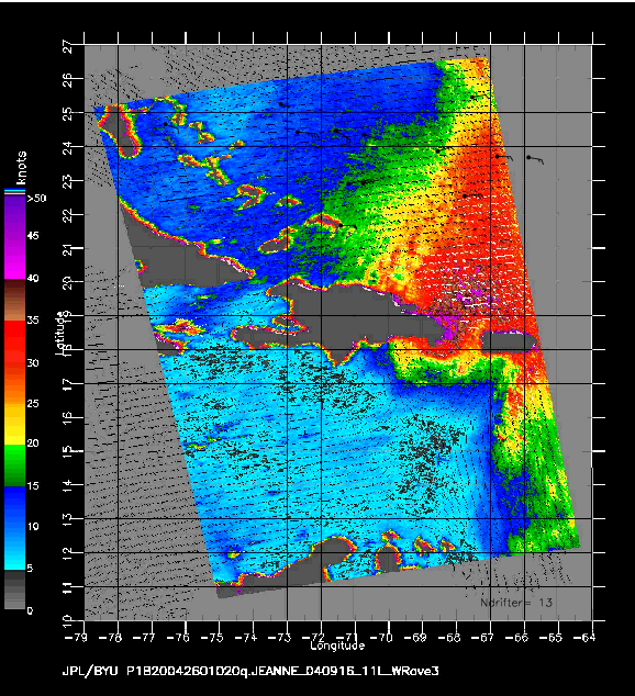
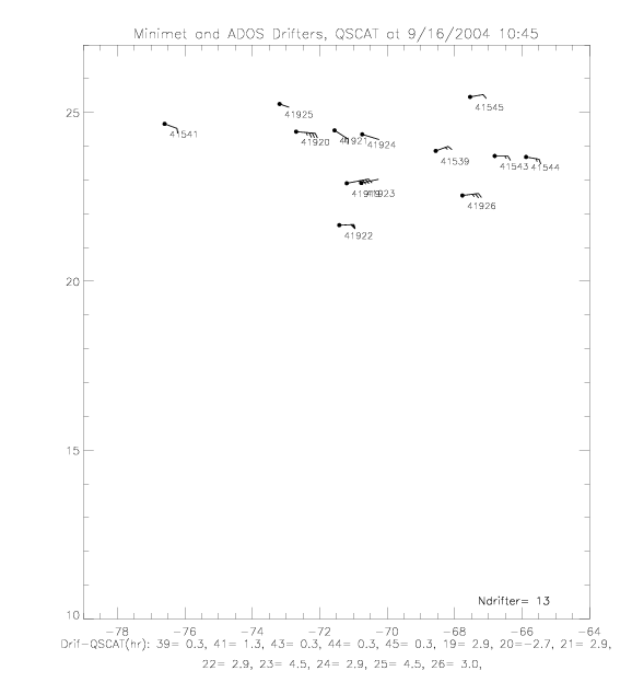 Fig. 1.1 9/16/2004 10:45 UTC, QSCAT high-res wind speed and drifter obs (a), and drifters obs only.
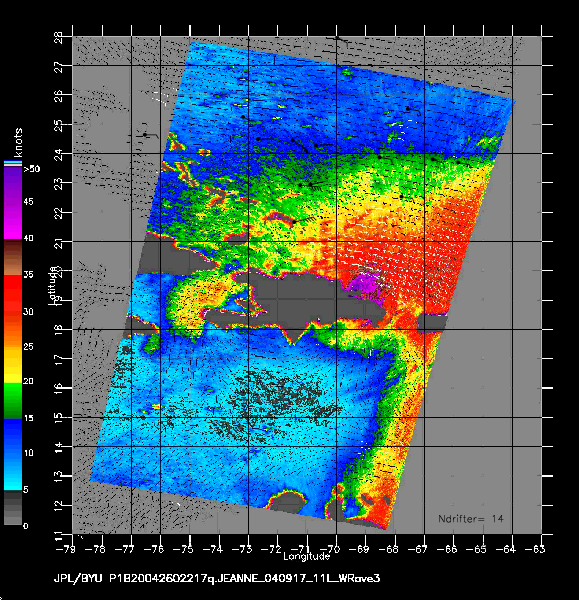
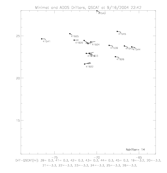 Fig. 1.2 9/16/2004 22:42 UTC, QSCAT high-res wind speed and drifter obs (a), and drifters obs only (b).
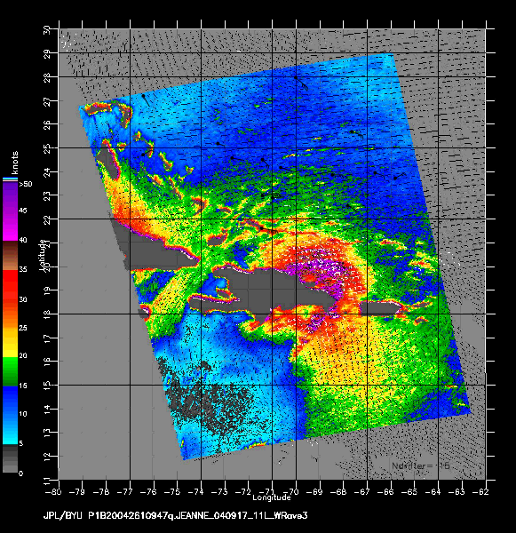
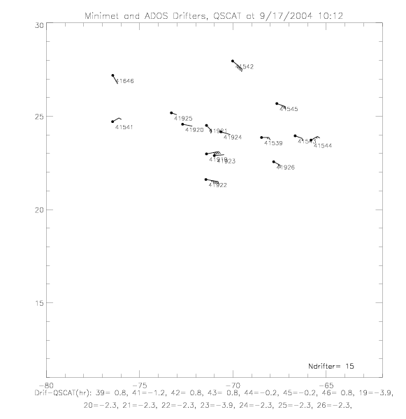 Fig. 1.3 9/17/2004 10:12 UTC, QSCAT high-res wind speed and drifter obs (a), and drifters obs only (b).
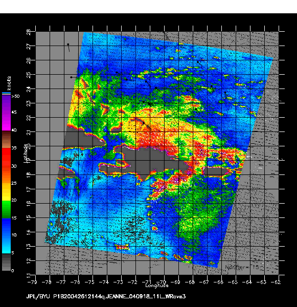
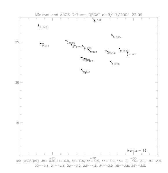 Fig. 1.4 9/17/2004 22:09 UTC, QSCAT high-res wind speed and drifter obs (a), and drifters obs only (b).
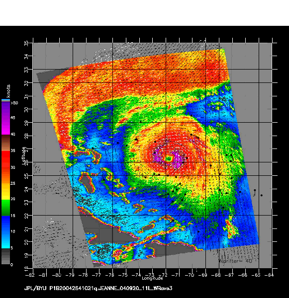
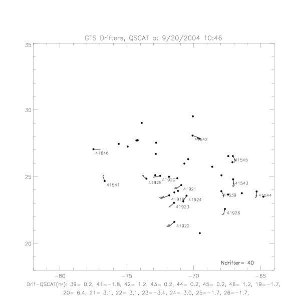 Fig. 1.5 9/20/2004 10:46 UTC, QSCAT high-res wind speed and drifter obs (a), and drifters obs only (b).
In fig.1.5 and following figures, the location of drifters with SST and air pressure measurements are also indicated,
in addition to drifters with wind direction and speed measurements.
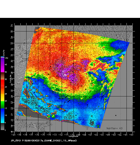
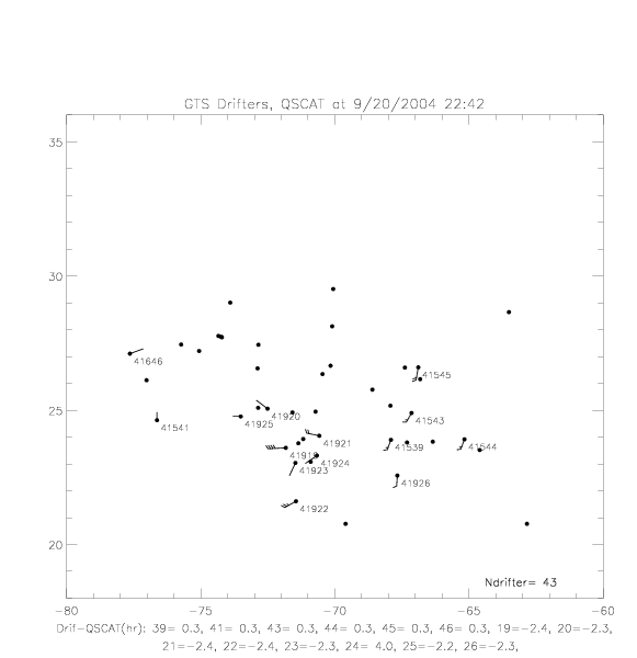 Fig. 1.6 9/20/2004 22:42 UTC, QSCAT high-res wind speed and drifter obs (a), and drifters obs only (b).
Drifters measured wind direction, wind speed, SST, and air pressure.
During the passage of hurricanes Frances and Jeanne, there were a total of 66 drifters with useful data in the area of roughly
280-300°E and 20-30°N: 9 Metocean (dir, speed, SST, pres), 8 ADOS (dir,speed,SST,pres),
14 Minimet (SST,pres), 12 SVP-15m (SST), 3 SVP-15m (SST,pres), 17 SST drifters (SST), and
3 SST&pres drifters (SST,pres).
Below are plots of the drifter tracks (based on GTS files), for the time period 8/25 - 10/1/2004. Open squares
indicate deployment locations (or beginning of data records), and dots indicate locations at end of
data records (with drifter labels). The tracks of Frances and Jeanne are superimposed, with dates and highest
recorded wind speeds (in m/s). Plots for each group of drifters follow below.
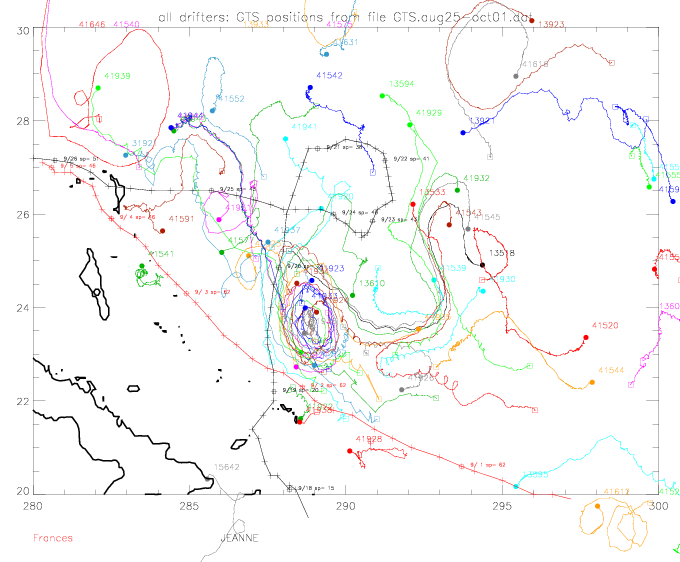 Fig. 2.1 All GTS drifter tracks, 8/25-10/1/2004, and tracks of Frances and Jeanne.
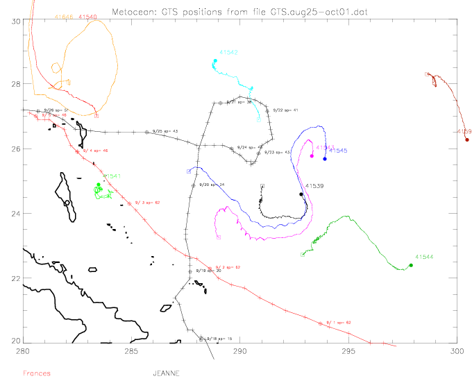
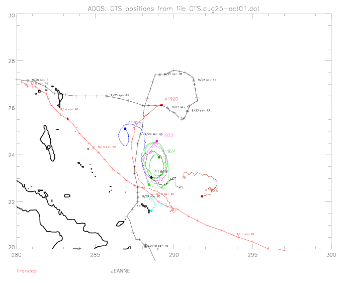 Fig. 2.2 Drifter tracks, 8/25-10/1/2004, for (a) Metocean, and (b) ADOS drifters.
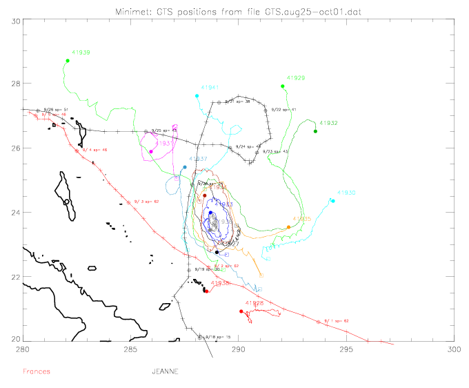
 Fig. 2.3 Drifter tracks, 8/25-10/1/2004, for (a) Minimet, and (b) SVP-15m drifters.
 Fig. 2.4 Drifter tracks, 8/25-10/1/2004, for (a) SVP-100m, and (b) SST drifters.
 Fig. 2.5 Drifter tracks, 8/25-10/1/2004, for SST&pres drifters.
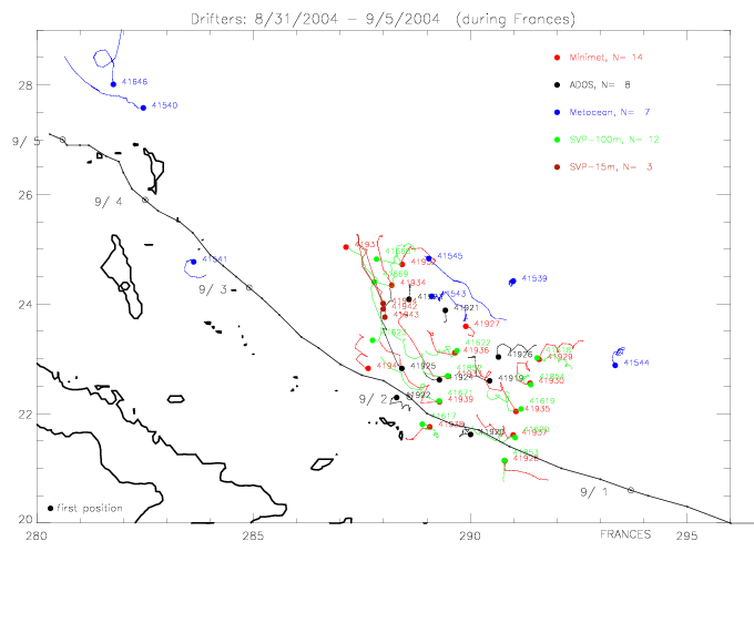 Fig. 2.6 Minimet, ADOS, Metocean, SVP-100m and SVP-15m drifter tracks, during Frances, 8/31-9/5/2004.
The drifter IDs, time period for observations, and type of observations for each drifter are summarized in
Table 2.1.
Table 2.1: List of all Drifters in Frances and Jeanne
| Type | Drifter | dates | days |
N dir | N speed | N SST | N pres |
| SST (17) | 13518 | 8/25-10/01 | 37 | | | 306 | |
| | 13594 | 8/25-10/01 | 37 | | | 318 | |
| | 13595 | 8/31-10/01 | 31 | | | 220 | |
| | 13608 | 8/25-09/24 | 30 | | | 244 | |
| | 13610 | 8/25-10/01 | 37 | | | 292 | |
| | 13921 | 8/25-10/01 | 37 | | | 341 | |
| | 13923 | 8/25-10/01 | 37 | | | 360 | |
| | 31921 | 8/25-10/01 | 37 | | | 335 | |
| | 41552 | 8/25-10/01 | 37 | | | 364 | |
| | 41554 | 8/25-10/01 | 37 | | | 333 | |
| | 41555 | 9/10-10/01 | 21 | | | 200 | |
| | 41559 | 9/10-10/01 | 21 | | | 199 | |
| | 41575 | 8/25-10/01 | 37 | | | 250 | |
| | 41577 | 8/25-10/01 | 37 | | | 363 | |
| | 41591 | 8/25-10/01 | 37 | | | 352 | |
| | 41612 | 8/25-10/01 | 37 | | | 319 | |
| | 41616 | 8/25-10/01 | 37 | | | 360 | |
| SST&pres (3) | 13533 | 8/25-10/01 | 37 | | | 880 | 879 |
| | 41520 | 8/25-10/01 | 37 | | | 1454 | 1454 |
| | 41631 | 8/25-10/01 | 37 | | | 535 | 537 |
| Metocean (9) | 41539 | 8/25-10/01 | 37 | 682 | 696 | 692 | 699 |
| | 41540 | 8/25-09/09 | 15 | 262 | 276 | 278 | 280 |
| | 41541 | 8/25-10/01 | 37 | 568 | 647 | 647 | 654 |
| | 41542 | 8/25-10/01 | 37 | 643 | 667 | 670 | 671 |
| | 41543 | 8/25-10/01 | 37 | 662 | 671 | 672 | 676 |
| | 41544 | 8/25-10/01 | 37 | 645 | 665 | 666 | 672 |
| | 41545 | 8/25-10/01 | 37 | 650 | 674 | 679 | 685 |
| | 41590 | 8/25-10/01 | 37 | 381 | | 642 | 641 |
| | 41646 | 8/25-10/01 | 37 | 511 | | 515 | 515 |
| ADOS (8) | 41919 | 8/31-10/01 | 30 | 193 | | 66 | 238 |
| | 41920 | 8/31-10/01 | 30 | 201 | | 227 | 240 |
| | 41921 | 9/04-10/01 | 27 | 196 | 207 | 56 | 209 |
| | 41922 | 9/01-10/01 | 30 | 232 | 251 | 218 | 250 |
| | 41923 | 9/03-10/01 | 28 | 131 | | 141 | 146 |
| | 41924 | 9/04-10/01 | 27 | 192 | | 316 | 215 |
| | 41925 | 9/01-10/01 | 30 | 228 | | 264 | 236 |
| | 41926 | 8/31-10/01 | 30 | 251 | | 338 | 259 |
| Minimet (14) | 41927 | 9/01-10/01 | 30 | | | 176 | 176 |
| | 41928 | 8/31-10/01 | 30 | | | 163 | 161 |
| | 41929 | 8/31-10/01 | 30 | | | 170 | 169 |
| | 41930 | 8/31-10/01 | 30 | | | | 156 |
| | 41931 | 9/04-10/01 | 26 | | | 133 | 134 |
| | 41932 | 9/01-10/01 | 30 | | | 161 | 160 |
| | 41933 | 8/31-10/01 | 30 | | | 159 | 159 |
| | 41934 | 9/01-10/01 | 30 | | | 181 | 180 |
| | 41935 | 9/01-10/01 | 30 | | | 176 | 177 |
| | 41936 | 9/01-10/01 | 30 | | | 186 | 188 |
| | 41937 | 8/31-10/01 | 30 | | | 177 | 176 |
| | 41938 | 8/31-09/15 | 14 | | | 75 | 76 |
| | 41939 | 8/31-10/01 | 30 | | | 168 | 169 |
| | 41941 | 8/31-10/01 | 30 | | | 188 | 186 |
| SVP-15m (3) | 41942 | 9/01-10/01 | 30 | | | 269 | 268 |
| | 41943 | 8/31-10/01 | 30 | | | 269 | 277 |
| | 41944 | 9/01-10/01 | 30 | | | 248 | 251 |
| SVP-100m (12) | 41617 | 8/31-10/01 | 30 | | | 336 | |
| | 41618 | 8/31-10/01 | 30 | | | 327 | |
| | 41619 | 8/31-10/01 | 30 | | | 313 | |
| | 41620 | 8/31-10/01 | 30 | | | 321 | |
| | 41622 | 8/31-10/01 | 30 | | | 312 | |
| | 41623 | 8/31-10/01 | 30 | | | 334 | |
| | 41668 | 8/31-10/01 | 30 | | | 338 | |
| | 41669 | 8/31-10/01 | 30 | | | 316 | |
| | 41671 | 8/31-10/01 | 30 | | | 314 | |
| | 41852 | 8/31-10/01 | 30 | | | 330 | |
| | 41853 | 8/31-10/01 | 30 | | | 132 | |
| | 41854 | 8/31-10/01 | 30 | | | 326 | |
A summary of number of drifters for each type of observation is listed in Tabel 2.2.
Not all drifter records extend to 10/1/2004: one SST drifter ends on 9/24, one Metocean ends on 9/9, and one Minimet ends on 9/15.
Table 2.2: Number of Drifters with Data
| Type | Total | dir | speed | SST | pres |
| SST | 17 | - | - | 17 | - |
| SST&pres | 3 | - | - | 3 | 3 |
| Metocean | 9 | 9 | 7 | 9 | 9 |
| ADOS | 8 | 8 | 2 | 8 | 8 |
| Minimet | 14 | - | - | 13 | 14 |
| SVP-15m | 3 | - | - | 3 | 3 |
| SVP-100m | 12 | - | - | 12 | - |
| | | | | | |
| Total | 66 | 17 | 9 | 65 | 37 |
The position data from the GTS website are compared with Pacific Gyre's data, i.e. with
GPS (in red) and ARGOS (in blue) positions. The plots below show ADOS drifters 41920 (WMO no. 37019)
and 41921 (WMO no. 37021). The difference between GTS and ARGOS positions seems to be simply in
the number of significant digits in the data files. There are only a few instances when the GPS
positions are very different from the GTS track. It ususally is due to extra GPS data during
time periods when there were no GTS data available and the GTS track was simply interpolated
between the nearest positions.
 Fig. 2.1.1 Position data from GTS, GPS, and ARGOS, for ADOS drifters (a) 41920, and (b) 41921.
Below are position plots for two Minimets: drifter 41932 (WMO no. 49578) and 41939 (WMO no. 49585).
The GPS data are more frequent, especially in the later part of the deployments; and they point to two instances
of erroneous GTS position data: for drifter 41932 at about (291°E, 23.5°N), and for 41939 at (282°E, 28°N).
The corrected GTS data are potted in fig. 2.7.
 Fig. 2.1.2 Position data from GTS (uncorrected), GPS, and ARGOS, for Minimet drifters (a) 41932,
and (b) 41939.
Fig. 2.1.2 Position data from GTS (uncorrected), GPS, and ARGOS, for Minimet drifters (a) 41932,
and (b) 41939.
 Fig. 2.1.3 Position data from GTS (corrected), GPS, and ARGOS, for Minimet drifters (a) 41932,
and (b) 41939.
Fig. 2.1.3 Position data from GTS (corrected), GPS, and ARGOS, for Minimet drifters (a) 41932,
and (b) 41939.
The next figure shows examples from quality-controlled data files, and GPS position data. The quality-controlled
data have position data only for valid wind, SST, or pressure observations.
 Fig. 2.1.4 Position data from quality-controlled data files and GPS, for Minimet drifters (a) 41927,
and (b) 41933.
Fig. 2.1.4 Position data from quality-controlled data files and GPS, for Minimet drifters (a) 41927,
and (b) 41933.
Nine Metocean drifters (ID 4139-45, 41590, and 41646) and eight ADOS drifters (ID 41919-41926).
In the following figures, "Time of observation", the drifter observations are plotted as day vs. hour of day: blck dots indicate position data only (possibly SST and pressure), blue indicates direction data available, and red means direction and speed available. Note, that QSCAT observations in the area of the drifters occur around 10:30 and 22:30.
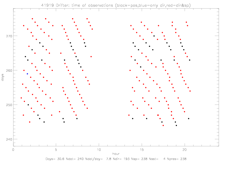
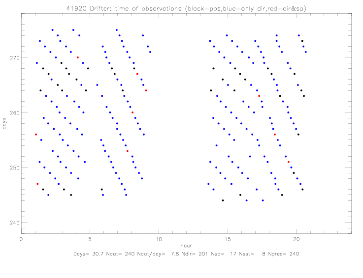 Fig. 3.1 Time of observations for ADOS drifters (a) 41919, and (b) 41920.
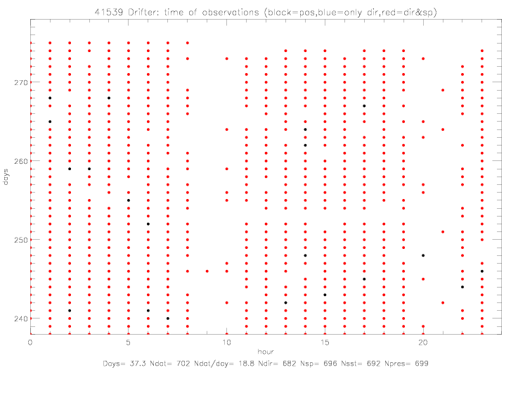
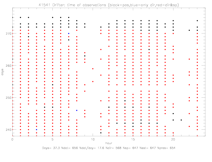 Fig. 3.2 Time of observations for Metocean drifters (a) 41539, and (b) 41541.
In the following figures, the "distance" panel shows distance between drifter and the center of the hurricane (AOML data),
speed shows drifter measured speeds, if available, in black, hurricane "maximum sustained winds" from AOML in blue, and
collocated QSCAT speeds (in red). The figures in this section are based on raw data, without any quality control.
The ADOS figures in this section do not contain any SST data. In section 5, quality controlled data are plotted, and
ADOS SST data from a secondary sensor.
Hurricane data are available every 3 hours, for almost the entire data period, and when missing were interpolated to
every 3 hours. 9 Metocean, 8 ADOS, 14 Minimet, 3 SVP-15m, 12 SVP-100m, 17 SST ,
and 3 SST&pres drifters are plotted below.
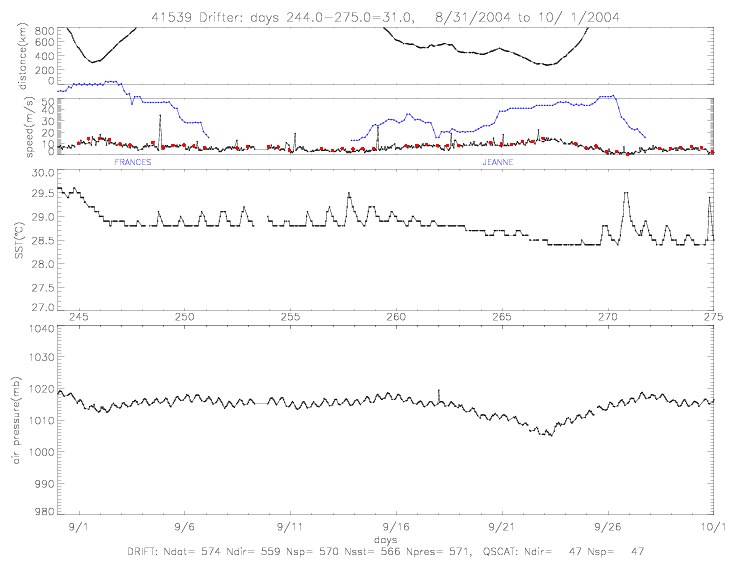
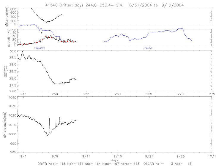 Fig. 4.1.1 Drifter wind speed, SST, and air pressure for Metocean drifters (a) 41539, and (b) 41540.
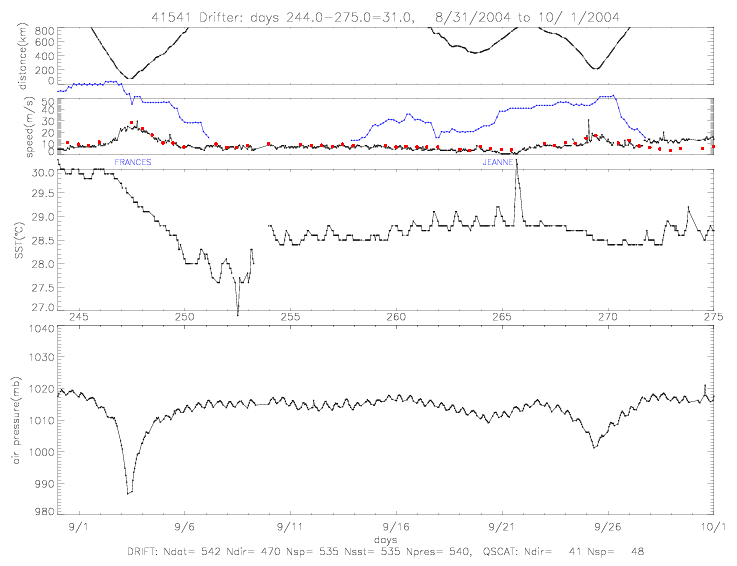
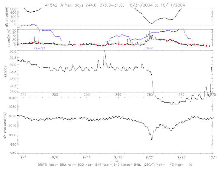 Fig. 4.1.2 Drifter wind speed, SST, and air pressure for Metocean drifters (a) 41541, and (b) 41542.
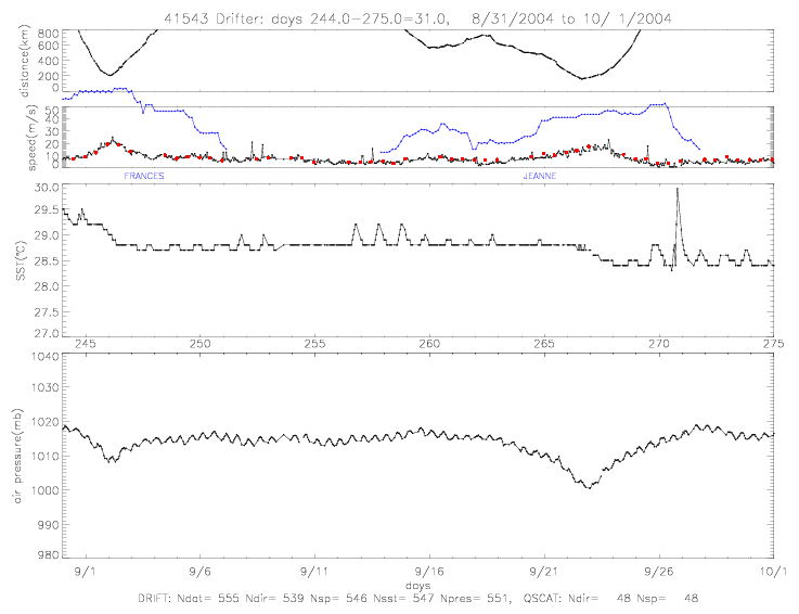
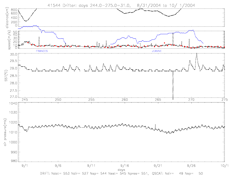 Fig. 4.1.3 Drifter wind speed, SST, and air pressure for Metocean drifters (a) 41543, and (b) 41544.
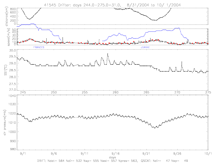
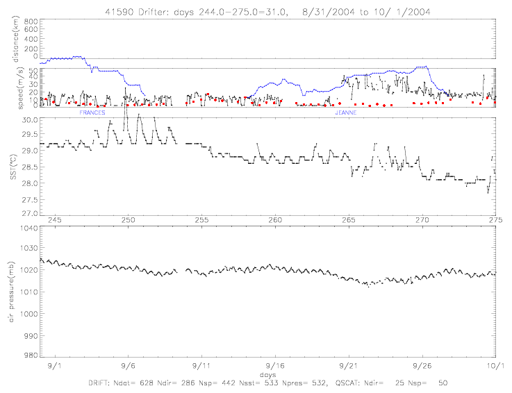 Fig. 4.1.4 Drifter wind speed, SST, and air pressure for Metocean drifters (a) 41545, and (b) 41590.
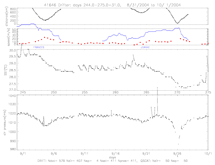 Fig. 4.1.5 Drifter wind speed, SST, and air pressure for Metocean drifter 41646.
These un-corrected data files do not contain any SST data. SST data is plotted
in section 5.2 .
Fig. 4.1.5 Drifter wind speed, SST, and air pressure for Metocean drifter 41646.
These un-corrected data files do not contain any SST data. SST data is plotted
in section 5.2 .
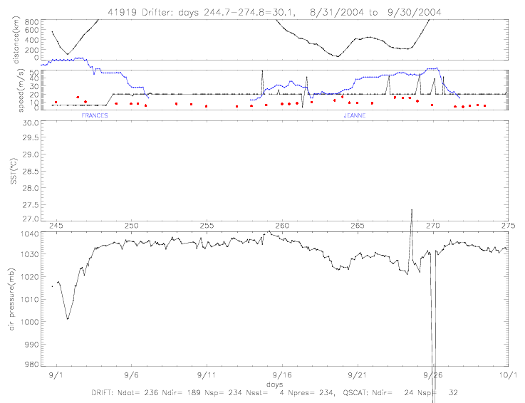
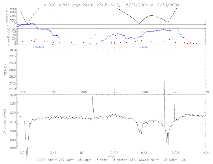 Fig. 4.2.1 Drifter wind speed, SST, and air pressure for ADOS drifters (a) 41919, and (b) 41920.
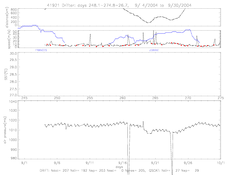
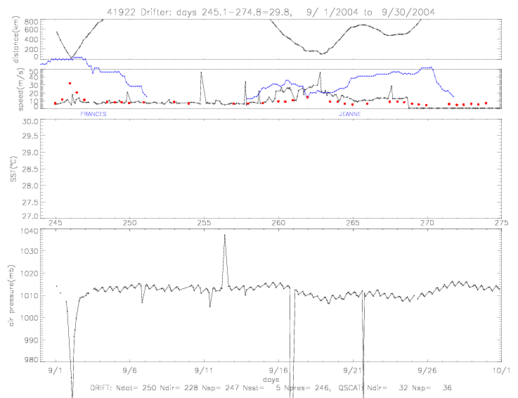 Fig. 4.2.2 Drifter wind speed, SST, and air pressure for ADOS drifters (a) 41921, and (b) 41922.
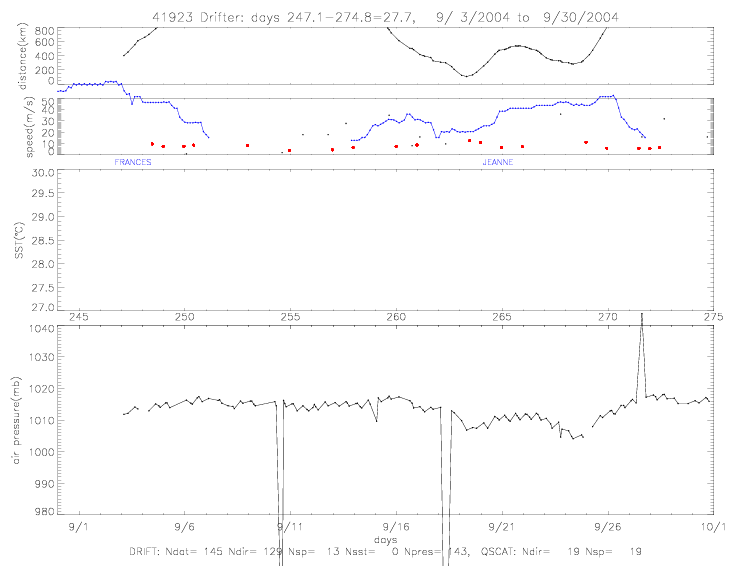
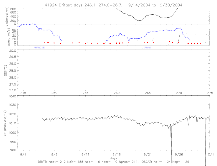 Fig. 4.2.3 Drifter wind speed, SST, and air pressure for drifter (a) 41923, and (b) 41924.
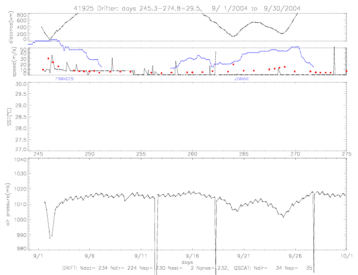
 Fig. 4.2.4 Drifter wind speed, SST, and air pressure for ADOS drifters (a) 41925, and (b) 41926.
There are several spikes in the pressure records of ADOS drifters, which need to be corrected.
The pressure records of six of the eight drifters agree very well with each other for time periods when the
drifters are not close to a hurricane. Two drifters, 41919 and 41922, seem to differ from all other
drifters by constant offsets. In the figures below, these two drifters are plotted together with drifter 41921
for comparison. Fig. 4.2.5b shows the pressure records after drifter 41919 has been corrected by subtracting 20mb,
and drifter 41922 has been corrected by adding 2mb.
 Fig. 4.2.5 Air pressure comparison for ADOS drifters 41921 with 41919 & 41922, (a) uncorrected, and (b) corrected.
In the plots with the corrected pressure, it is easy to correlate decreases in pressure with
distances to hurricanes. For example, at 9/1 and 9/2, when hurricane
Frances first approaches drifter 41919 (as close as 113km), the drifter records a drop
of air pressure to about 980mb. About 8hr later, the hurricane approaches drifter 41922
(as close as 20km), and here the pressure drops to 955mb.
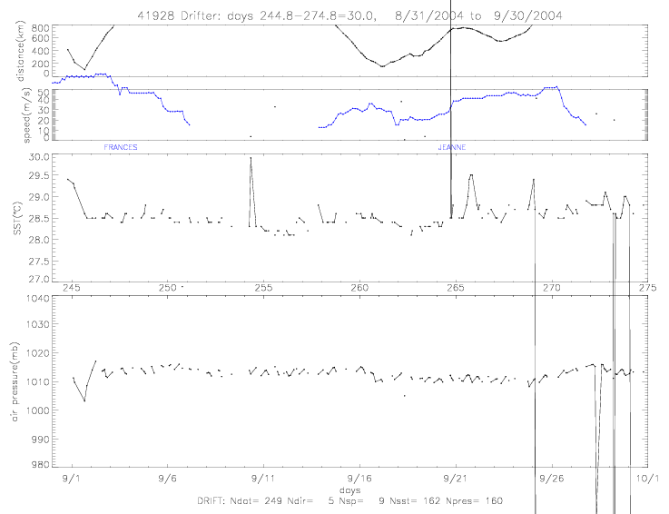 Fig. 4.3.1 Drifter SST and air pressure for Minimet drifters (a) 41927, and (b) 41928.
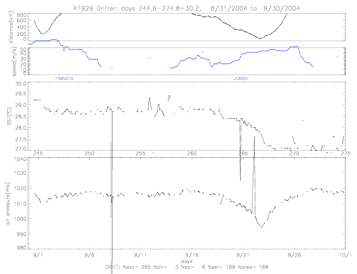
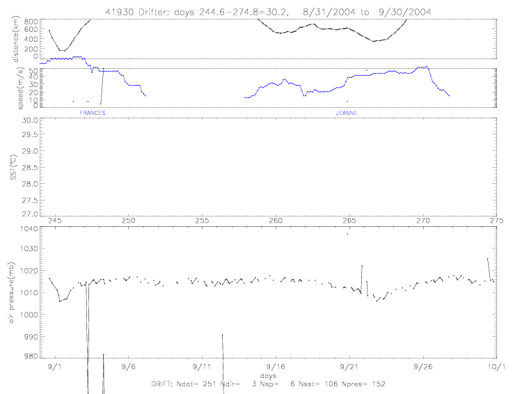 Fig. 4.3.2 Drifter SST and air pressure for Minimet drifters (a) 41929, and (b) 41930.
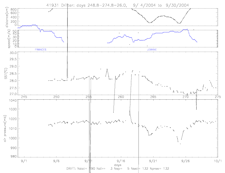
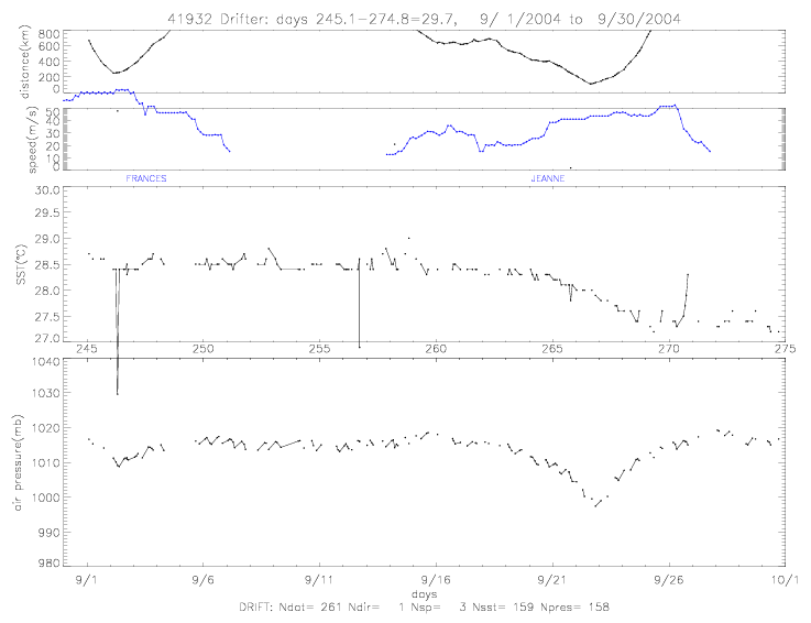 Fig. 4.3.3 Drifter SST and air pressure for Minimet drifters (a) 41931, and (b) 41932.
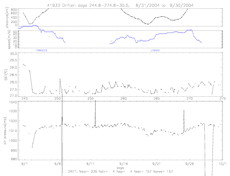
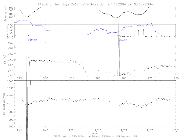 Fig. 4.3.4 Drifter SST and air pressure for Minimet drifters (a) 41933, and (b) 41934.
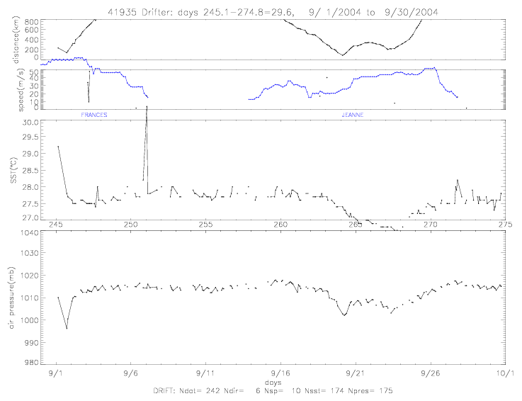
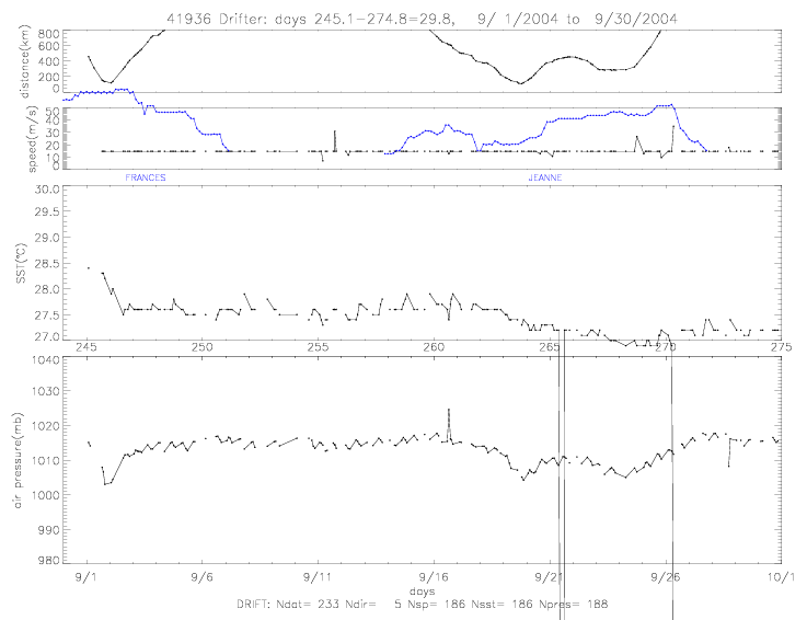 Fig. 4.3.5 Drifter SST and air pressure for Minimet drifters (a) 41935, and (b) 41936.
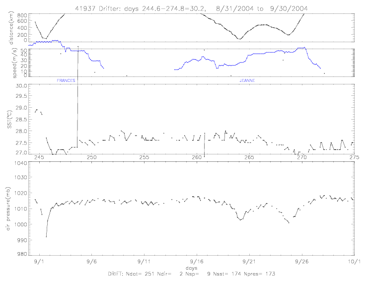
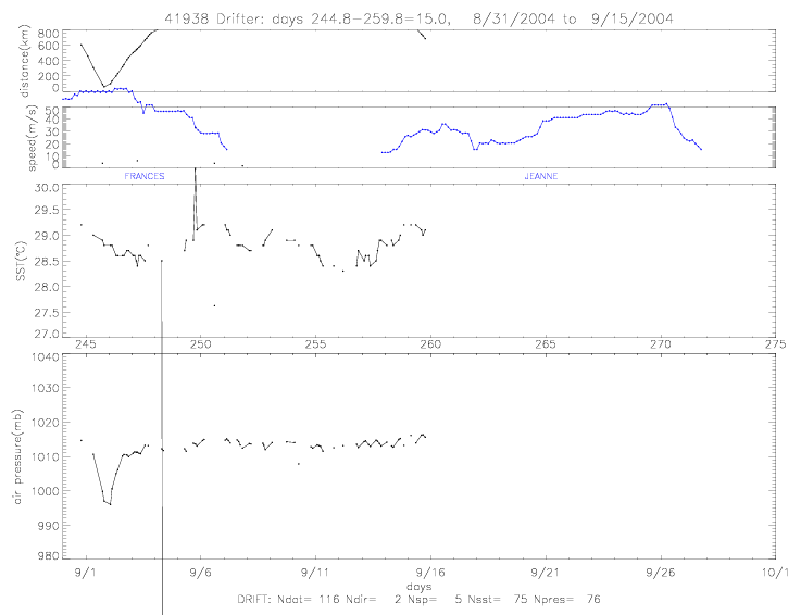 Fig. 4.3.6 Drifter SST and air pressure for Minimet drifters (a) 41937, and (b) 41938.
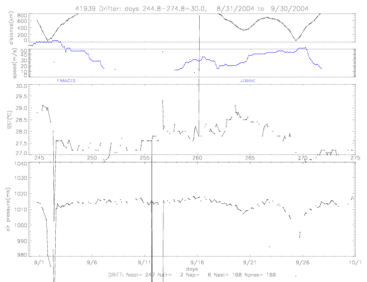
 Fig. 4.3.7 Drifter SST and air pressure for Minimet drifters (a) 41939, and (b) 41941.
 Fig. 4.4.1 Drifter SST and air pressure for SVP-15m drifters (a) 41942, and (b) 41943.
 Fig. 4.4.2 Drifter SST and air pressure for SVP-15m drifter 41944.
The three SVP-15m drifters stayed very close together after the deployment. Their SST observations
are not the same, however, but differ by offsets on the order of 0.3-1.2°C. The next figures show
the comparissons between the drifters. Plotted in each figure are time series of two drifters,
the SST difference of the two, the separation distance (in km), and the 2D plot of the two drifter
tracks. North and East directions are indicated, the length of each (50km) provide the scale
for the tracks.
 Fig. 4.4.3 SST comparison between SVP-15m (a) 41943 & 41944, and (b) 41943 & 41942.
The distance between the drifters is plotted, as well as the 2D tracks.
Fig. 4.4.3 SST comparison between SVP-15m (a) 41943 & 41944, and (b) 41943 & 41942.
The distance between the drifters is plotted, as well as the 2D tracks.
 Fig. 4.4.4 SST comparison between SVP-15m 41944 & 41942.
12 of 14 deployed SVP-100m drifters have usable SST observations.
Fig. 4.4.4 SST comparison between SVP-15m 41944 & 41942.
12 of 14 deployed SVP-100m drifters have usable SST observations.
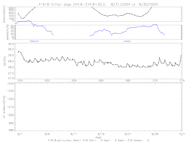 Fig. 4.5.1 Drifter SST for SVP-100m drifters (a) 41617, and (b) 41618.
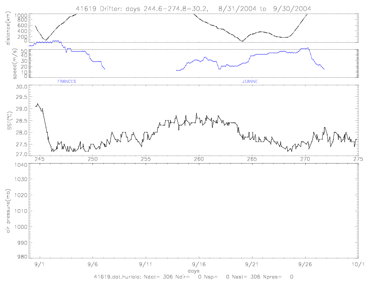
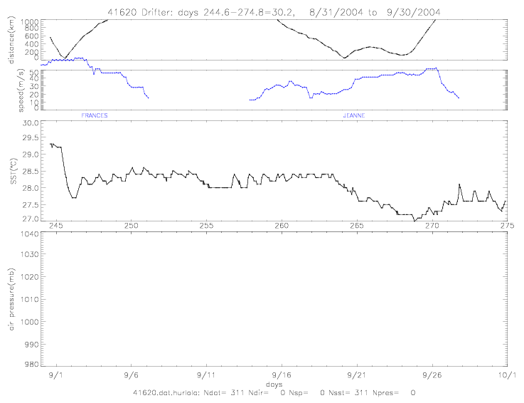 Fig. 4.5.2 Drifter SST for SVP-100m drifters (a) 41619, and (b) 41620.
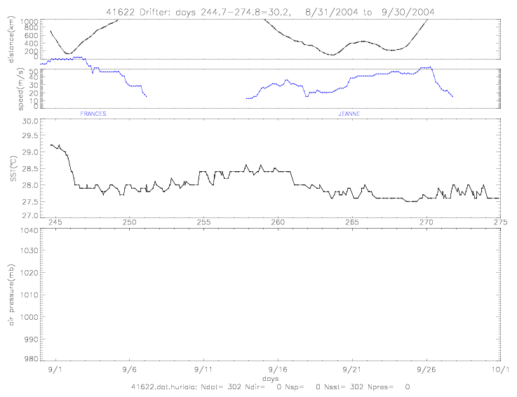
 Fig. 4.5.3 Drifter SST for SVP-100m drifters (a) 41622, and (b) 41623.
 Fig. 4.5.4 Drifter SST for SVP-100m drifters (a) 41668, and (b) 41669.
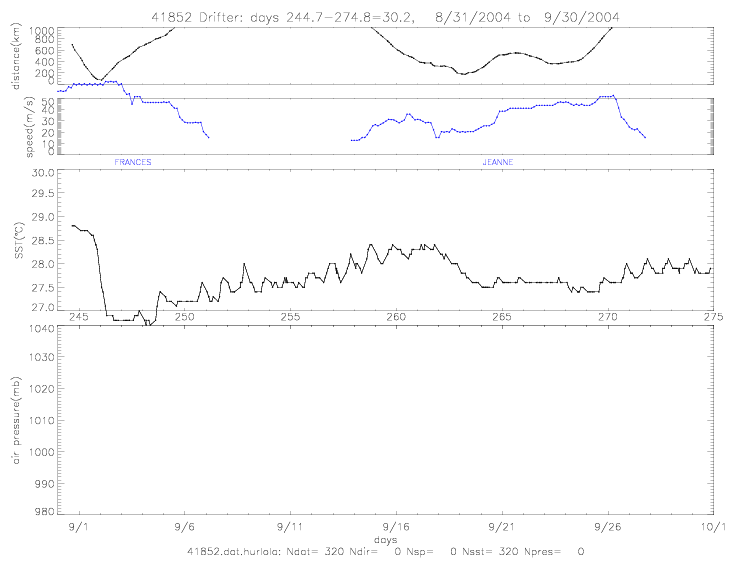 Fig. 4.5.5 Drifter SST for SVP-100m drifters (a) 41671, and (b) 41852.
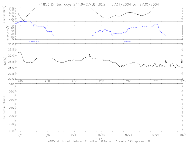
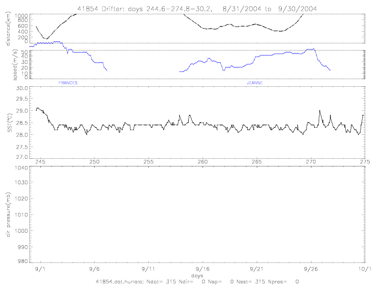 Fig. 4.5.6 Drifter SST for SVP-100m drifters (a) 41853, and (b) 41854.
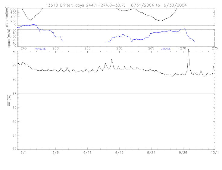
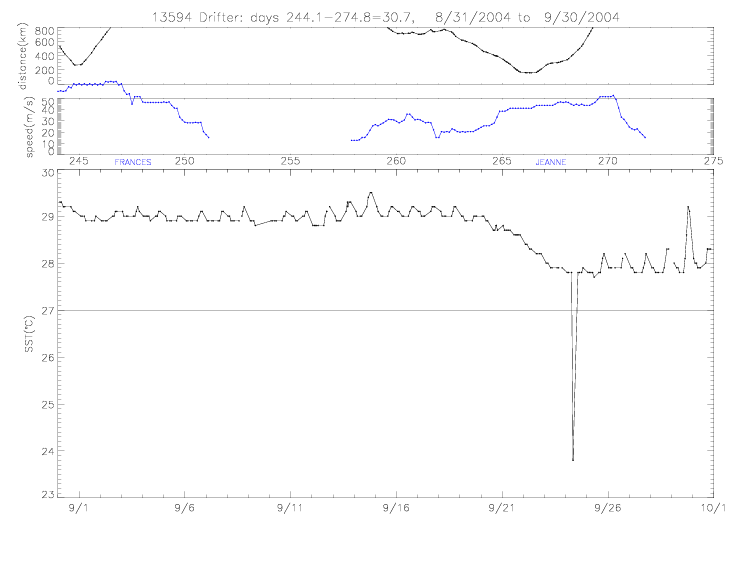 Fig. 4.6.1 Drifter SST for SST drifters (a) 13518, and (b) 13594.
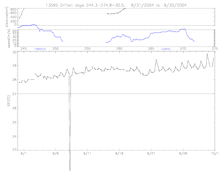
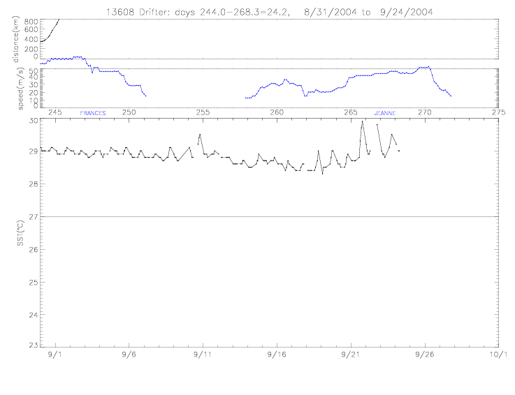 Fig. 4.6.2 Drifter SST for SST drifters (a) 13595, and (b) 13608.
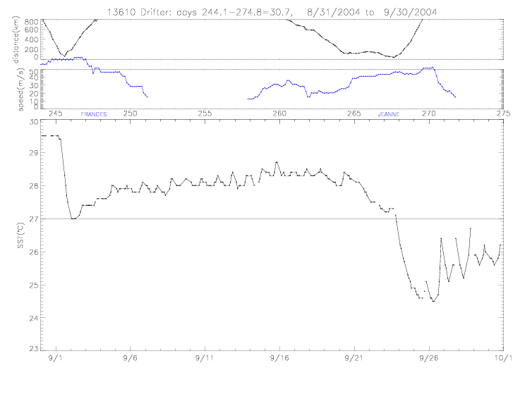
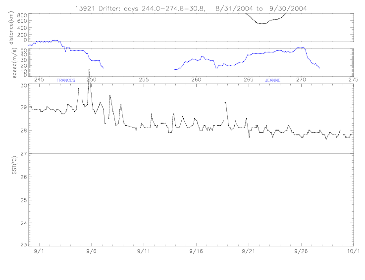 Fig. 4.6.3 Drifter SST for SST drifters (a) 13610, and (b) 13921.
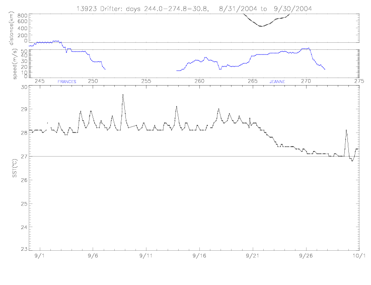
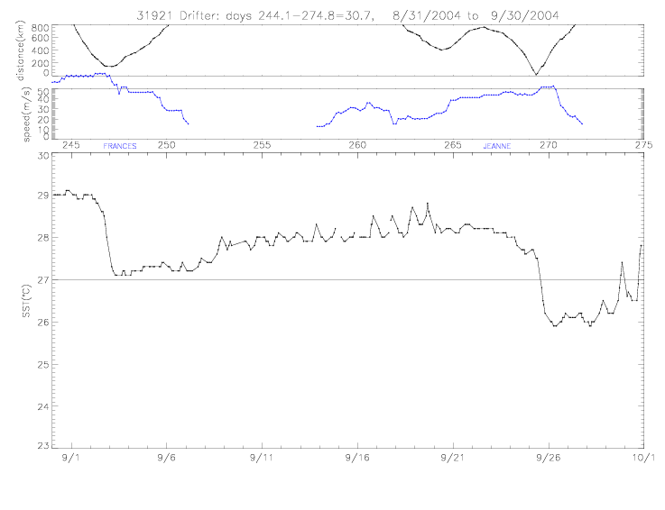 Fig. 4.6.4 Drifter SST for SST drifters (a) 13923, and (b) 31921.
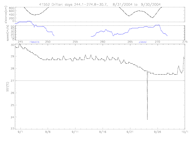
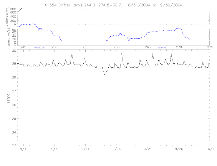 Fig. 4.6.5 Drifter SST for SST drifters (a) 41552, and (b) 41554.
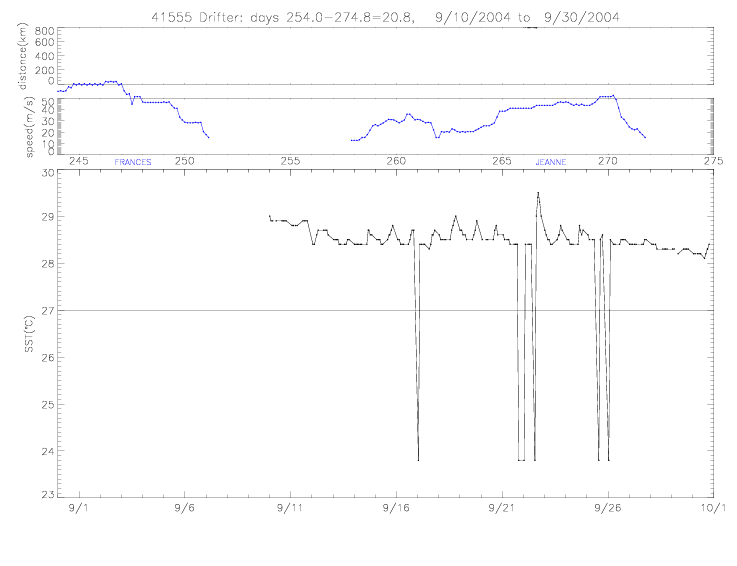
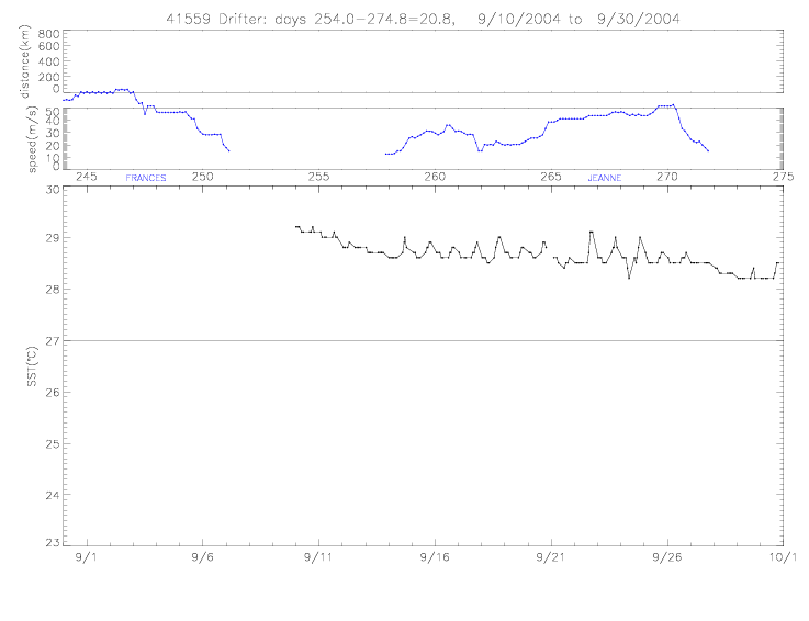 Fig. 4.6.6 Drifter SST for SST drifters (a) 41555, and (b) 41559.
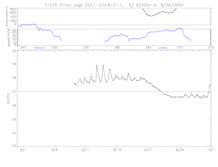
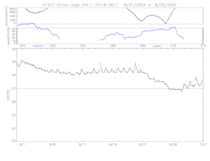 Fig. 4.6.7 Drifter SST for SST drifters (a) 41575, and (b) 41577.
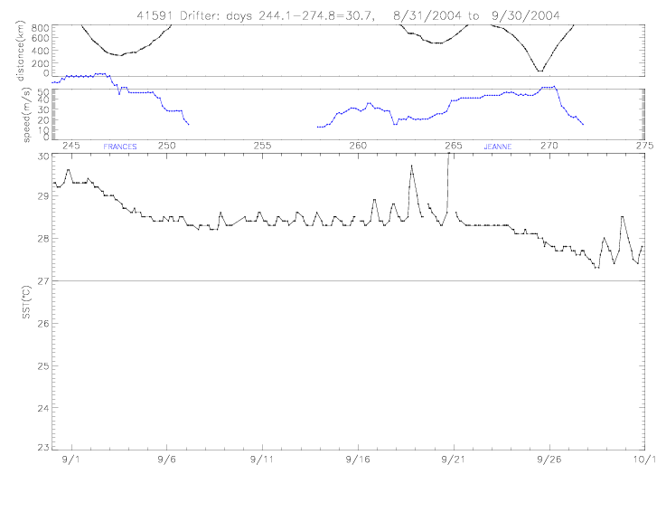
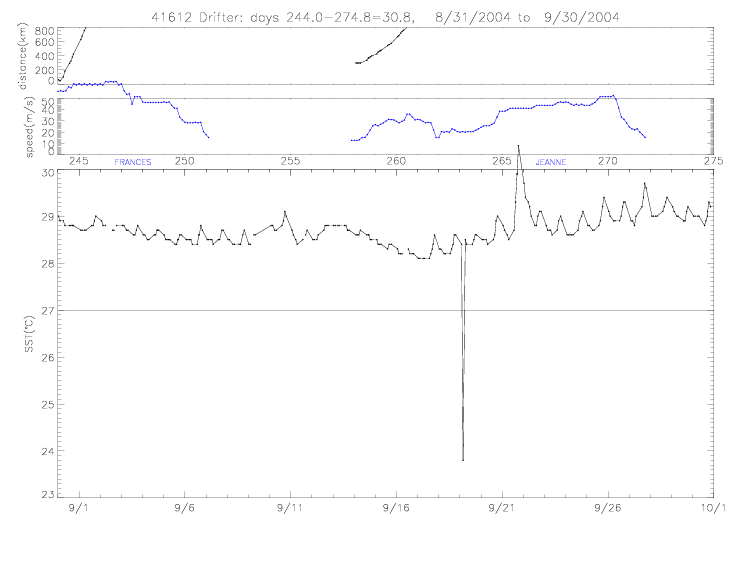 Fig. 4.6.8 Drifter SST for SST drifters (a) 41591, and (b) 41612.
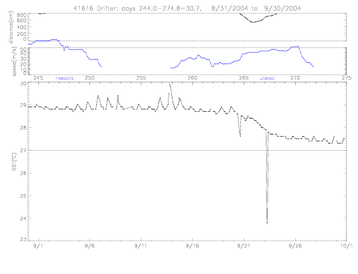 Fig. 4.6.9 Drifter SST for SST drifter 41616.
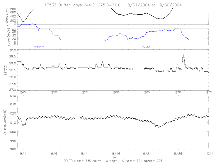
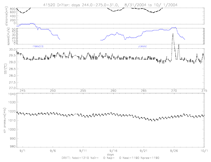 Fig. 4.7.1 Drifter SST and air pressure for SST&pres drifters (a) 13533, and (b) 41520.
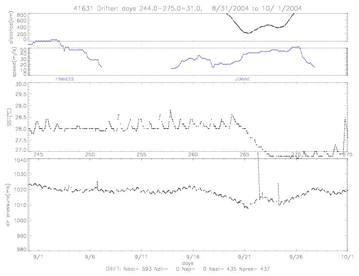 Fig. 4.7.2 Drifter SST and air pressure for SST&pres drifter 41631.
When comparing drifter time series of air pressure or SST, it becomes apparent that those
records agree mostly very well in the time period between the hurricanes, but differ from
each other during close encounters with the hurricanes - the differences depend on the distance
from the hurricane center. There are some drifters, however, that need to be corrected by small
offsets to align their records better with the records of all other drifters. The applied air
pressure offsets are only 1 to 3mb (except for drifter 41919, which requires a -20mb offset).
SST corrections vary between 0.1 and 1.6°C, but are mostly in the order of +/- 0.3°C.
In addition, there are a few obvious spikes that can be removed. Those corrections have been applied
to the data shown below (sections 5.1 - 5.6). The SST corrections are considered
preliminary, as it is planned to compute offsets from comparisons of drifter data with collocated satellite
SST observations.
For the figures below, Pacific Gyre data have been used for ADOS and Minimet drifters.
In contrast to GTS data files, these files contain more frequent data. During each successful
data transmission, the drifters transmit records from four 15min sampling intervals.
Pacific Gyre data files contain all those records, whereas GTS data files reflect only the
most recent data from each transmission.
A few spikes in SST, pressure, and speed were removed, and pressure was corrected for the following drifters:
41539 (-1mb), 41542 (-2mb), 41545 (-1mb), and 41590 (-3mb).
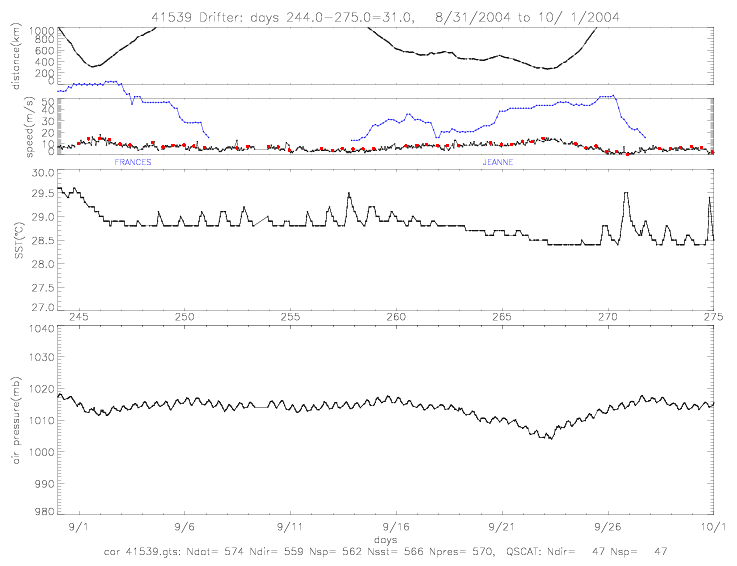
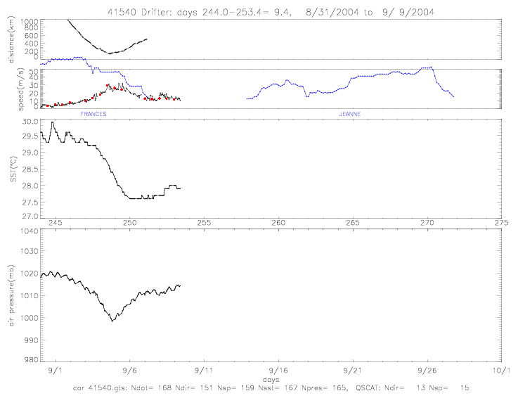 Fig. 5.1.1 Corrected drifter wind speed, SST, and air pressure for Metocean drifters (a) 41539, and (b) 41540.
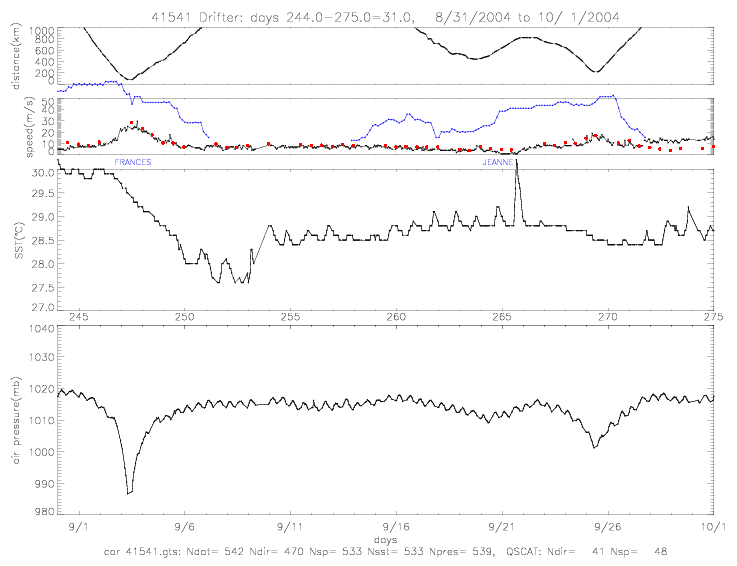
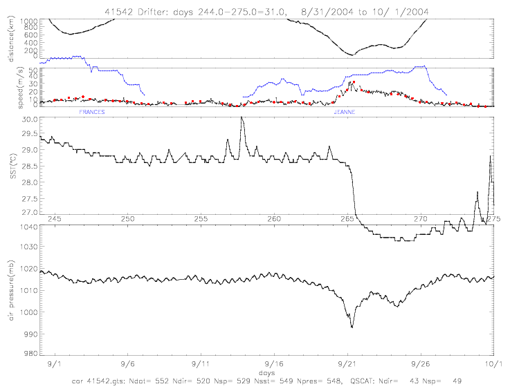 Fig. 5.1.2 Corrected drifter wind speed, SST, and air pressure for Metocean drifters (a) 41541, and (b) 41542.
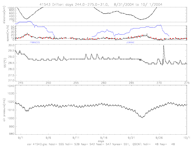
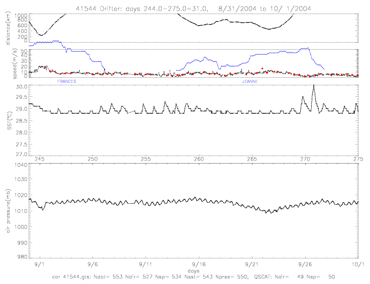 Fig. 5.1.3 Corrected drifter wind speed, SST, and air pressure for Metocean drifters (a) 41543, and (b) 41544.
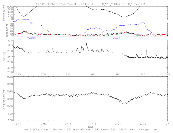
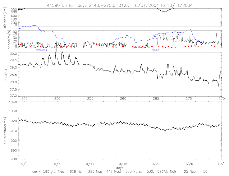 Fig. 5.1.4 Corrected drifter wind speed, SST, and air pressure for Metocean drifters (a) 41545, and (b) 41590.
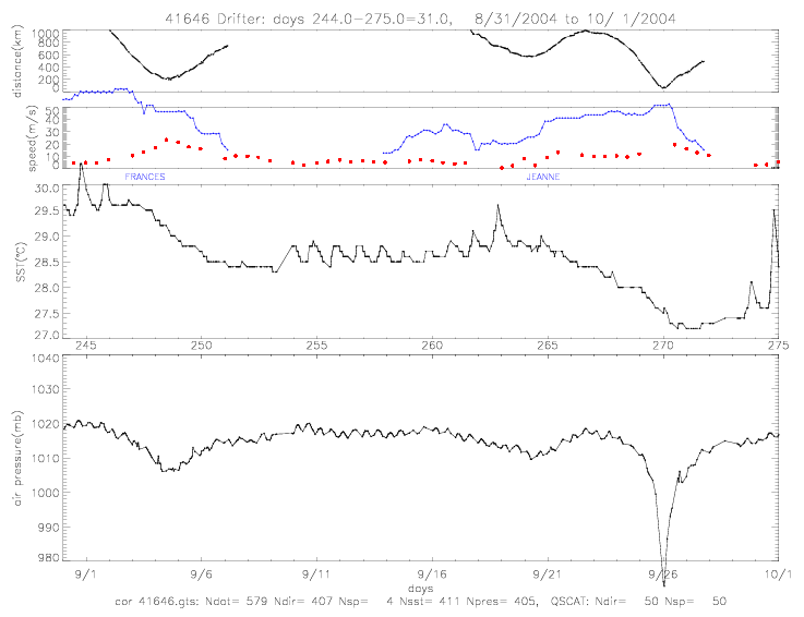 Fig. 5.1.5 Corrected drifter wind speed, SST, and air pressure for Metocean drifter 41646.
The corrected ADOS figures include SST data from a secondary sensor. Pressure was corrected for the
following drifters: 41919 (-20mb) and 41922 (-2mb).
Fig. 5.1.5 Corrected drifter wind speed, SST, and air pressure for Metocean drifter 41646.
The corrected ADOS figures include SST data from a secondary sensor. Pressure was corrected for the
following drifters: 41919 (-20mb) and 41922 (-2mb).
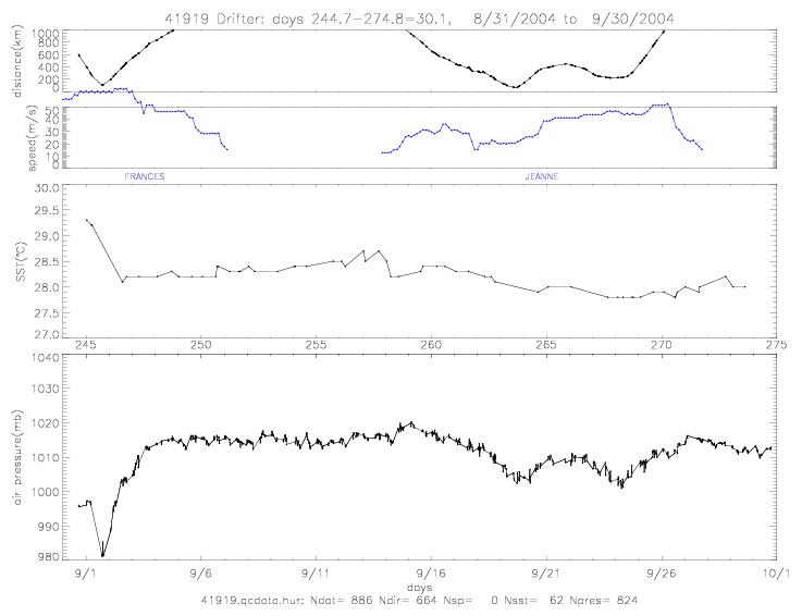
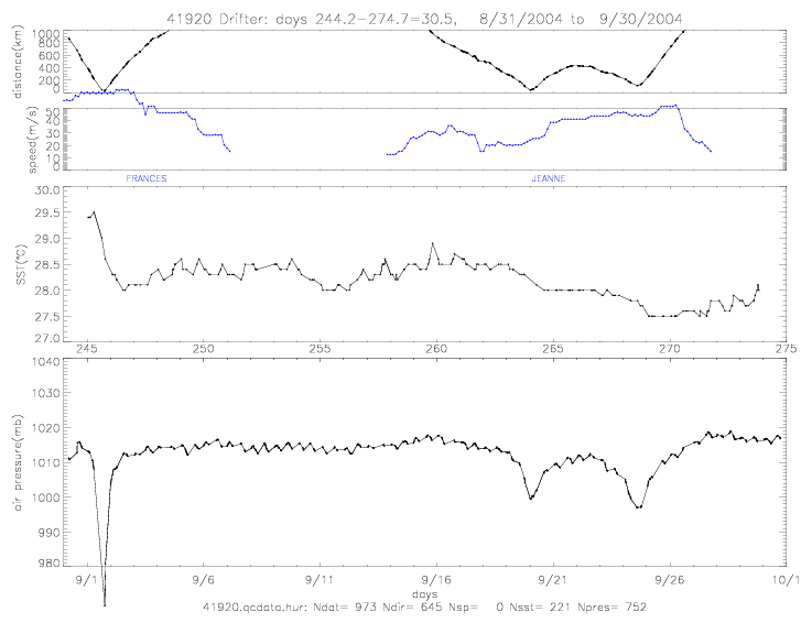 Fig. 5.2.1 Corrected drifter wind speed, SST, and air pressure for ADOS drifters (a) 41919, and (b) 41920.
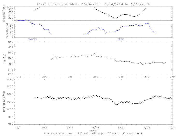
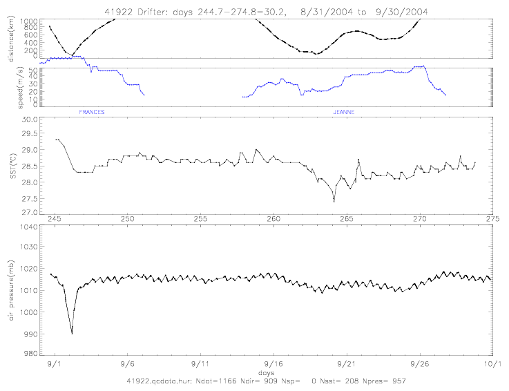 Fig. 5.2.2 Corrected drifter wind speed, SST, and air pressure for ADOS drifters (a) 41921, and (b) 41922.
 Fig. 5.2.3 Corrected drifter wind speed, SST, and air pressure for drifter (a) 41923, and (b) 41924.
 Fig. 5.2.4 Corrected drifter wind speed, SST, and air pressure for ADOS drifters (a) 41925, and (b) 41926.
A few spikes in SST and pressure were removed, and pressure was corrected for the following drifters:
41928 (+1mb), 41931 (-1mb), and 41939 (+1mb).

 Fig. 5.3.1 Corrected drifter SST and air pressure for Minimet drifters (a) 41927, and (b) 41928.
 Fig. 5.3.2 Corrected drifter SST and air pressure for Minimet drifters (a) 41929, and (b) 41930.
 Fig. 5.3.3 Corrected drifter SST and air pressure for Minimet drifters (a) 41931, and (b) 41932.
 Fig. 5.3.4 Corrected drifter SST and air pressure for Minimet drifters (a) 41933, and (b) 41934.
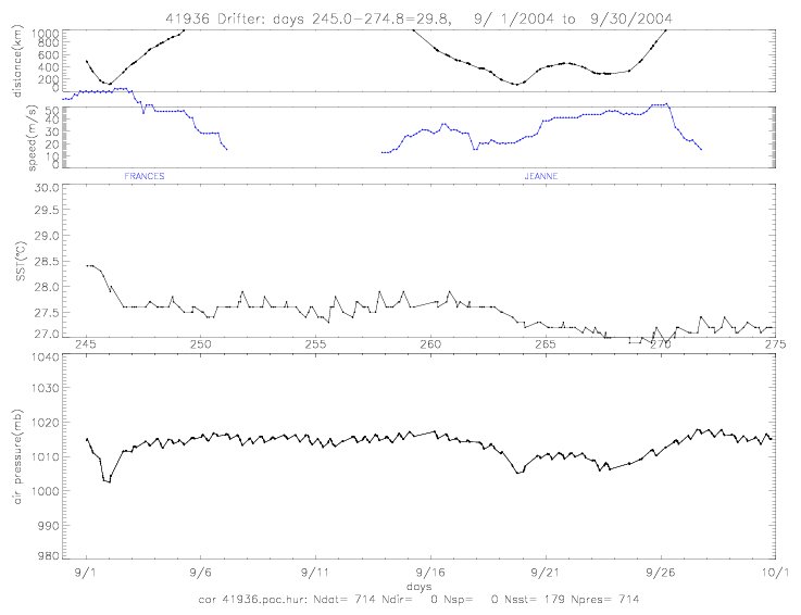 Fig. 5.3.5 Corrected drifter SST and air pressure for Minimet drifters (a) 41935, and (b) 41936.
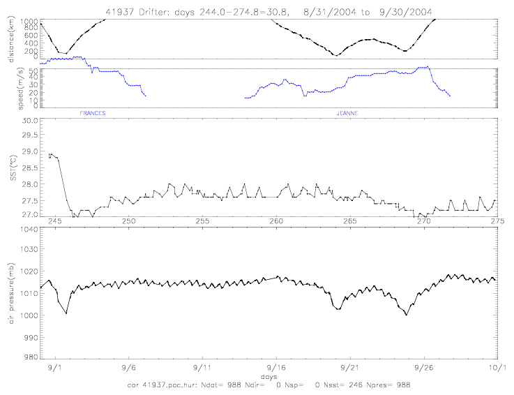
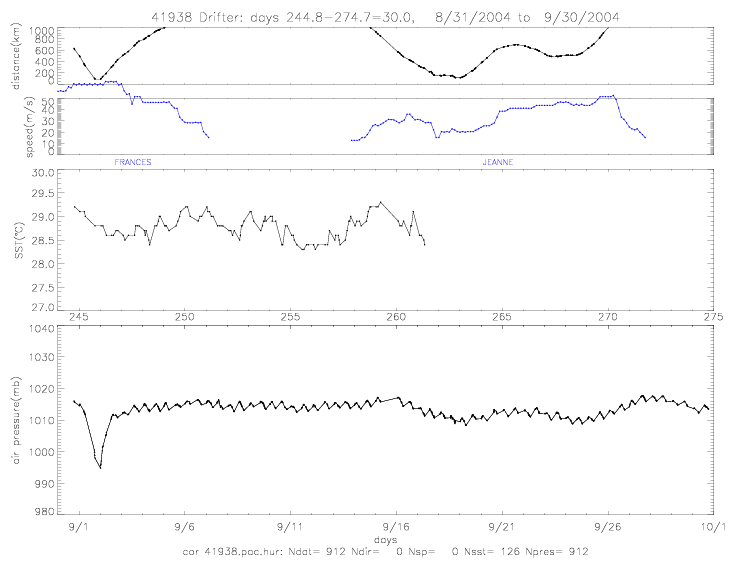 Fig. 5.3.6 Corrected drifter SST and air pressure for Minimet drifters (a) 41937, and (b) 41938.
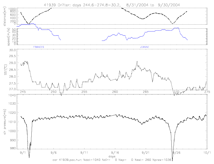
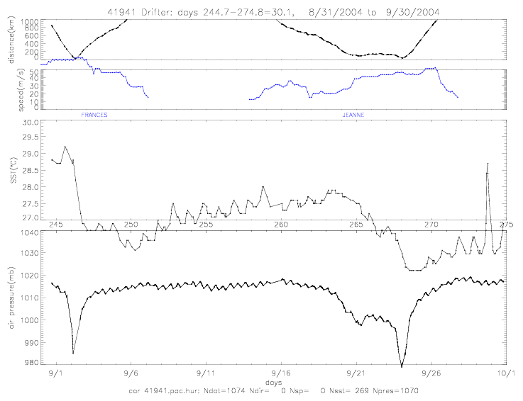 Fig. 5.3.7 Corrected drifter SST and air pressure for Minimet drifters (a) 41939, and (b) 41941.
All three SVP-15m drifters stayed very close together during Frances and Jeanne. It is not possibly to decide which drifter(s)
is the "truth", but the records can be corrected so that there are no offsets among these three drifters. The initial SST
from drifter 41942 is closest to other surrounding drifters (Metocean, ADOS, and Minimet), and was used to correct
the two drifters. Drifters 41943 and 41944 have also sudden shifts in their SST records that were corrected.
These shifts resulted from the SST measurement cycle, which was too short to get a correct SST reading.
Drifter 41943 was corrected by +1.2°C before day 249.0, and by +0.6°C afterwards.
Drifter 41944 was corrected by +0.8°C before day 260.5, and by +0.4°C afterwards.
Fig. 5.3.7 Corrected drifter SST and air pressure for Minimet drifters (a) 41939, and (b) 41941.
All three SVP-15m drifters stayed very close together during Frances and Jeanne. It is not possibly to decide which drifter(s)
is the "truth", but the records can be corrected so that there are no offsets among these three drifters. The initial SST
from drifter 41942 is closest to other surrounding drifters (Metocean, ADOS, and Minimet), and was used to correct
the two drifters. Drifters 41943 and 41944 have also sudden shifts in their SST records that were corrected.
These shifts resulted from the SST measurement cycle, which was too short to get a correct SST reading.
Drifter 41943 was corrected by +1.2°C before day 249.0, and by +0.6°C afterwards.
Drifter 41944 was corrected by +0.8°C before day 260.5, and by +0.4°C afterwards.
In addition, a few spikes were removed in SST and all pressure data were shifted by -1mb to become similar
to other neighboring drifters.
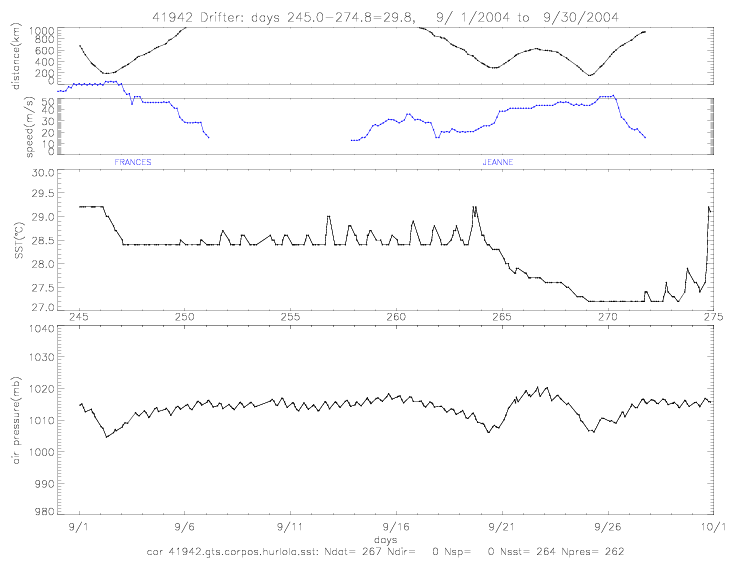
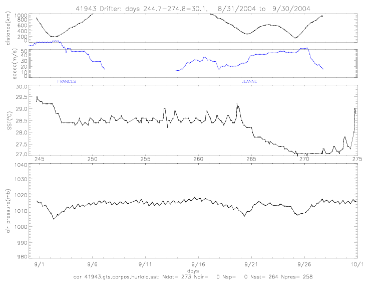 Fig. 5.4.1 Corrected drifter SST and air pressure for SVP-15m drifters (a) 41942, and (b) 41943.
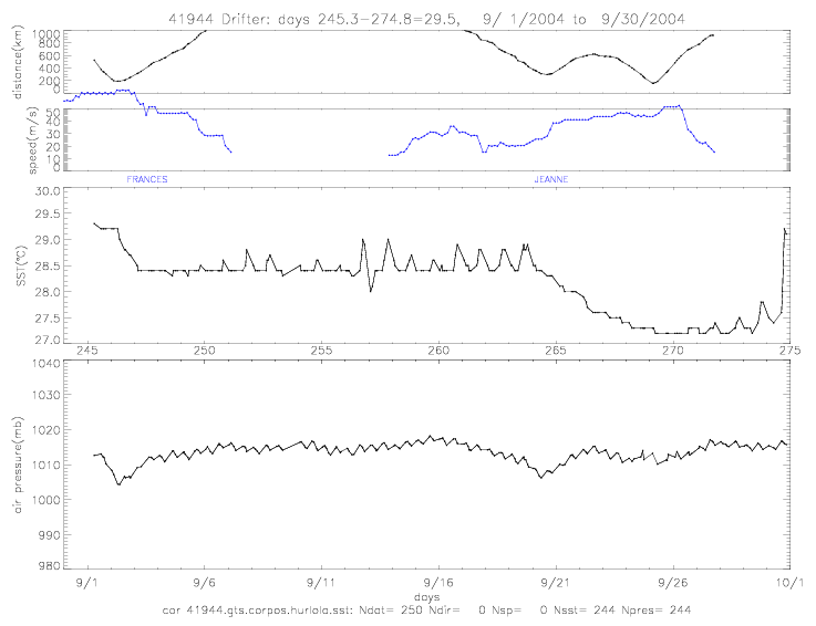 Fig. 5.4.2 Corrected drifter SST and air pressure for SVP-15m drifter 41944.
No corrections were applied to the SVP-100m SST data files. SST data are plotted
in section 4.5 .
Only very few SST spikes were removed in the SST drifters.
Fig. 5.4.2 Corrected drifter SST and air pressure for SVP-15m drifter 41944.
No corrections were applied to the SVP-100m SST data files. SST data are plotted
in section 4.5 .
Only very few SST spikes were removed in the SST drifters.
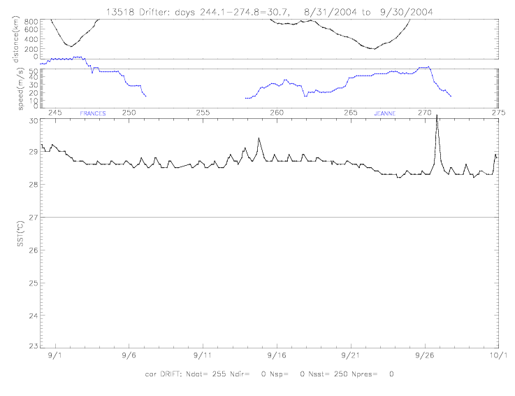
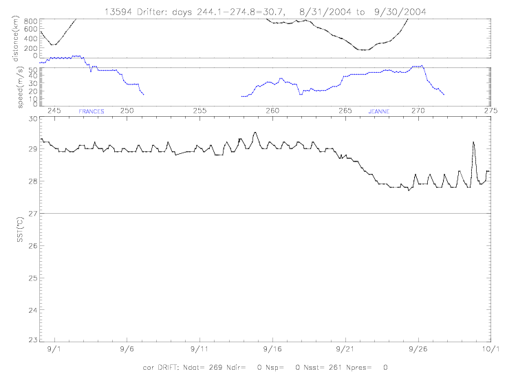 Fig. 5.6.1 Corrected drifter SST for SST drifters (a) 13518, and (b) 13594.
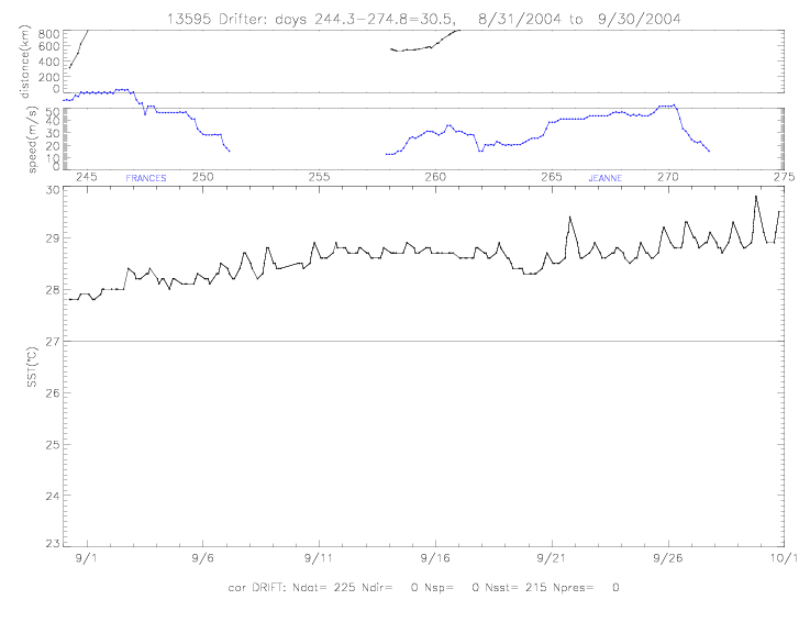
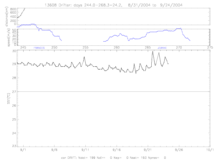 Fig. 5.6.2 Corrected drifter SST for SST drifters (a) 13595, and (b) 13608.
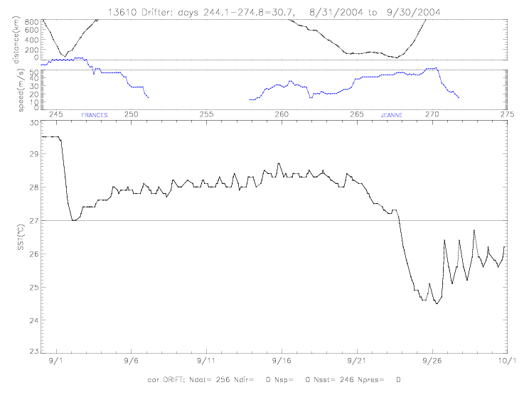
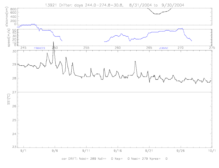 Fig. 5.6.3 Corrected drifter SST for SST drifters (a) 13610, and (b) 13921.
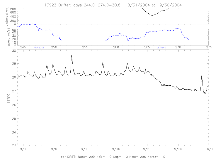
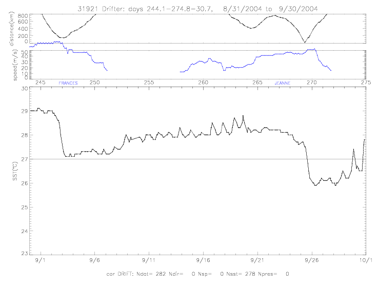 Fig. 5.6.4 Corrected drifter SST for SST drifters (a) 13923, and (b) 31921.
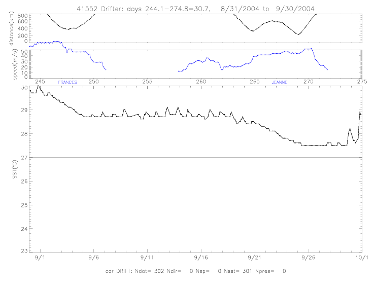
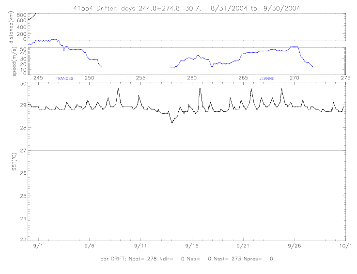 Fig. 5.6.5 Corrected drifter SST for SST drifters (a) 41552, and (b) 41554.
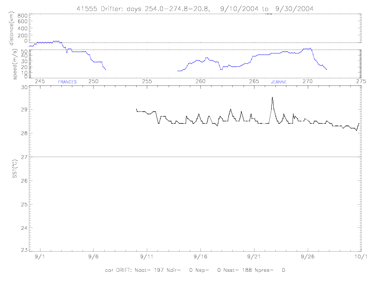
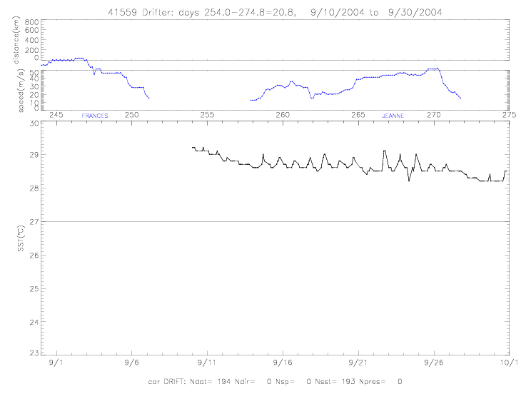 Fig. 5.6.6 Corrected drifter SST for SST drifters (a) 41555, and (b) 41559.
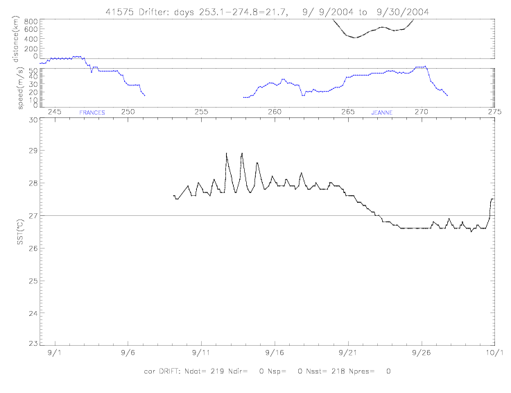
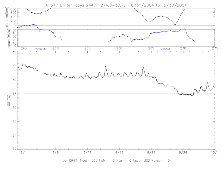 Fig. 5.6.7 Corrected drifter SST for SST drifters (a) 41575, and (b) 41577.
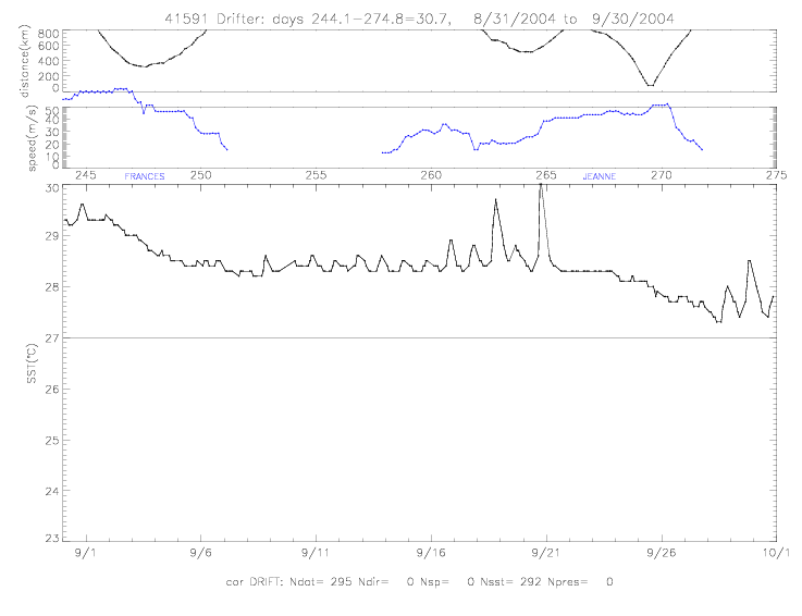
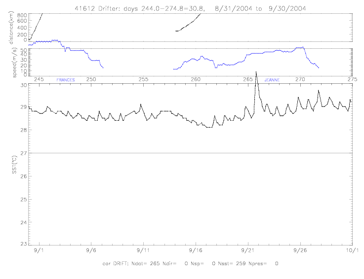 Fig. 5.6.8 Corrected drifter SST for SST drifters (a) 41591, and (b) 41612.
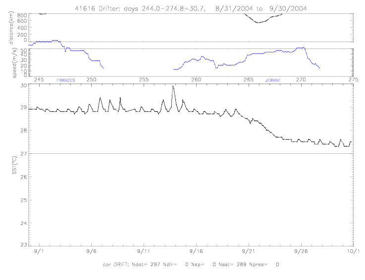 Fig. 5.6.9 Corrected drifter SST for SST drifter 41616.
A few spikes in SST and pressure were removed, and pressure was corrected for only one drifter:
41631 (-3mb).
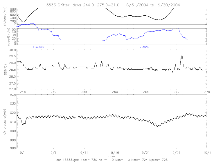
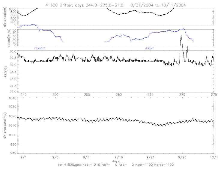 Fig. 5.7.1 Corrected drifter SST and air pressure for SST&pres drifters (a) 13533, and (b) 41520.
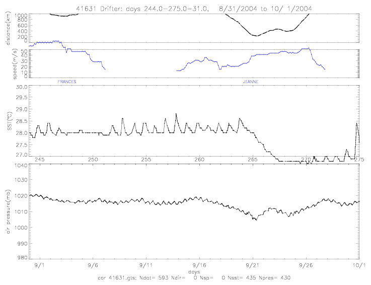 Fig. 5.7.2 Corrected drifter SST and air pressure for SST&pres drifter 41631.
The following figures are as above, but rain-flagged collocated QSCAT data are marked with open squares.
 Fig. 6.1 Drifter wind speed and direction for Metocean drifters (a) 41539, and (b) 41540.
 Fig. 6.2 Drifter wind speed and direction for Metocean drifters (a) 41541, and (b) 41542.
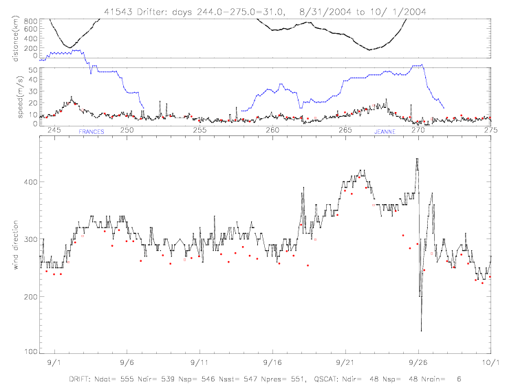
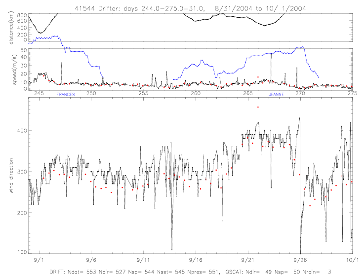 Fig. 6.3 Drifter wind speed and direction for Metocean drifters (a) 41543, and (b) 41544.
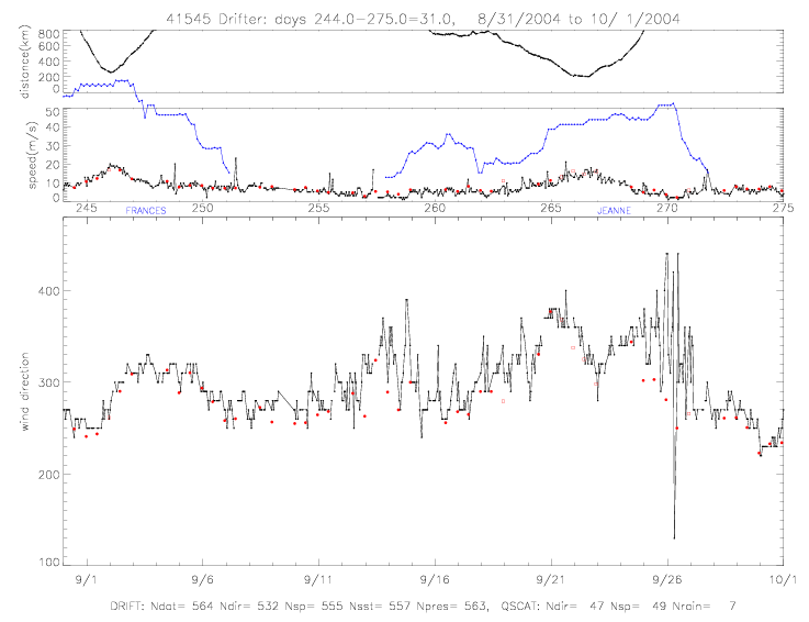
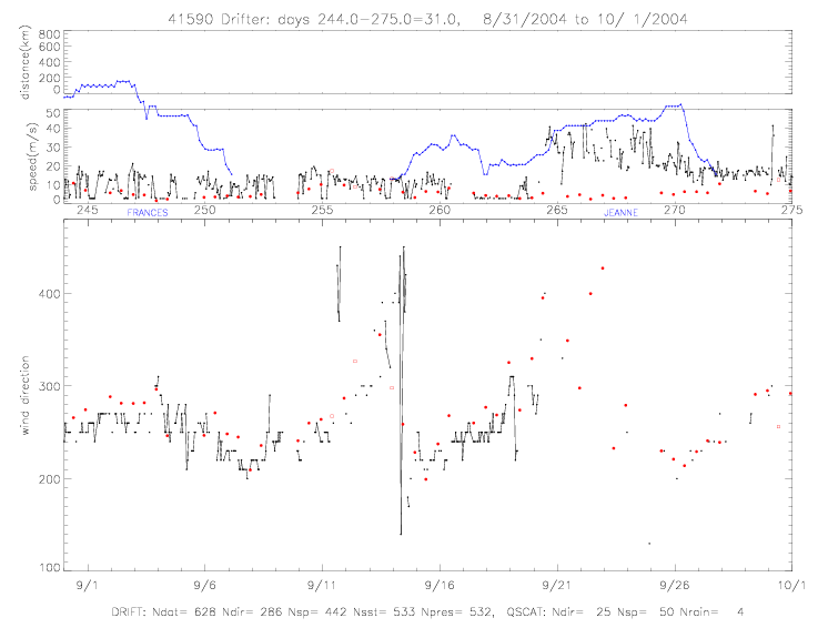 Fig. 6.4 Drifter wind speed and direction for Metocean drifters (a) 41545, and (b) 41590.
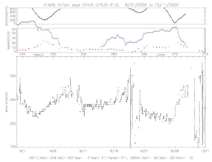 Fig. 5.5 Drifter wind speed and direction for Metocean drifter 41646.
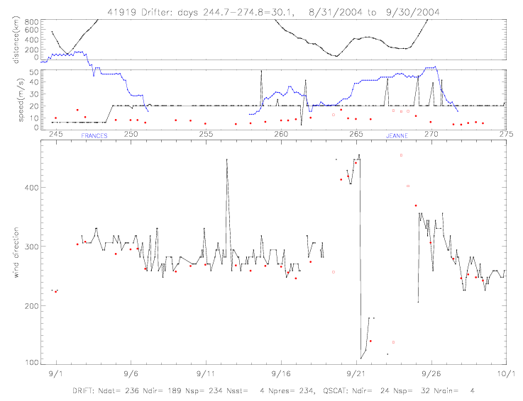
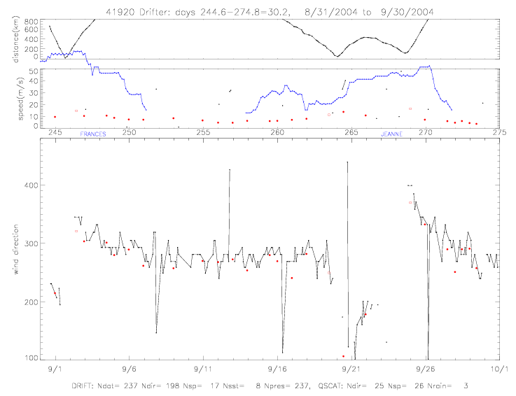 Fig. 6.6 Drifter wind speed and direction for ADOS drifters (a) 41919, and (b) 41920.
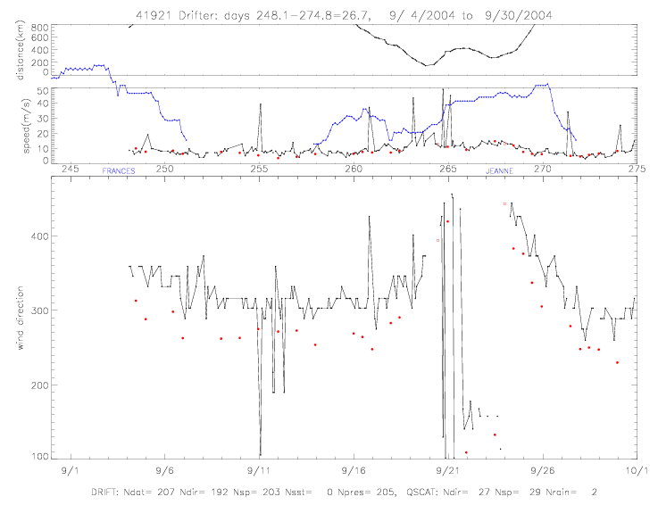
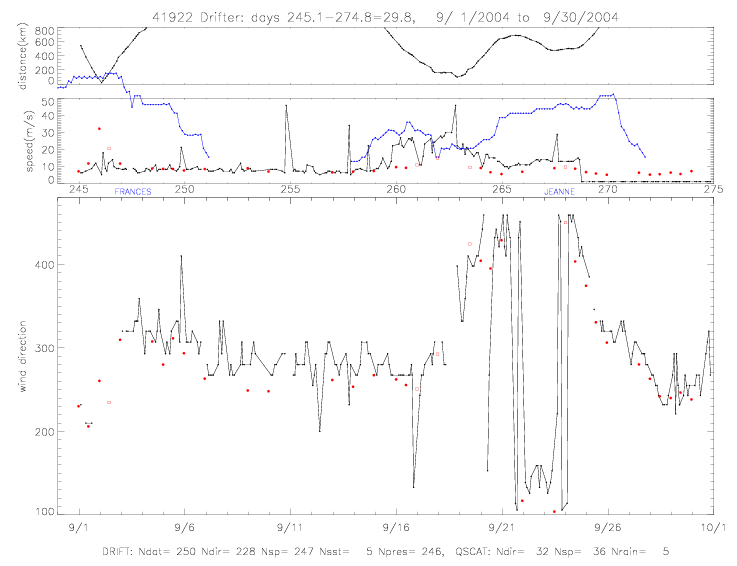 Fig. 6.7 Drifter wind speed and direction for ADOS drifters (a) 41921, and (b) 41922.
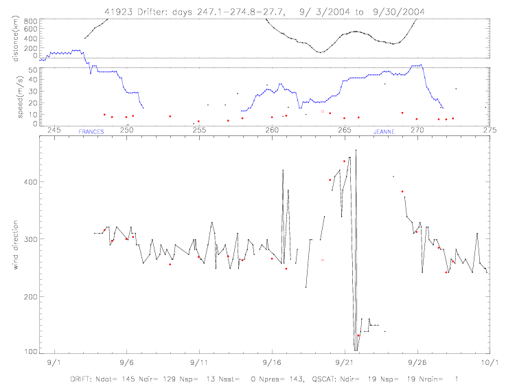
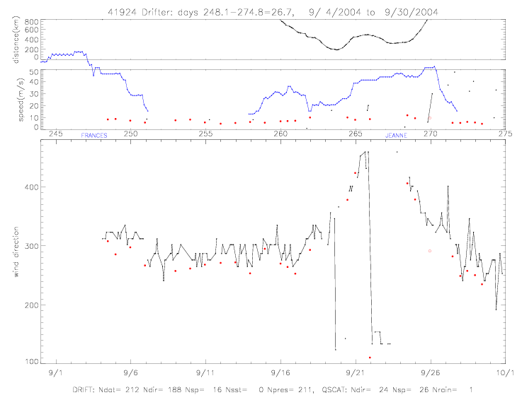 Fig. 6.8 Drifter wind speed and direction for ADOS drifters (a) 41923, and (b) 41924.
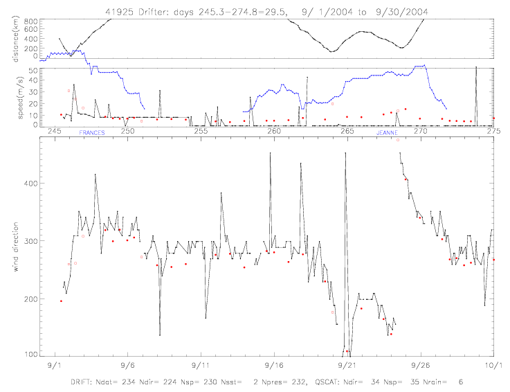
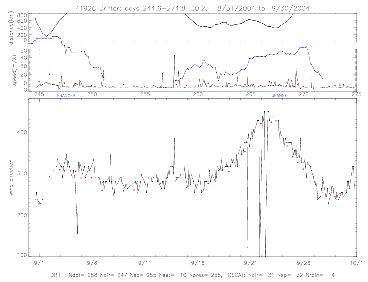 Fig. 6.9 Drifter wind speed and direction for ADOS drifters (a) 41925, and (b) 41926.
In the following figures, the differences between the GTS data (so far presented in previous figures) and data
from Pacific Gyre (PG, in green) are explored. Hurricane distances and speeds, as well as collocated QSCAT
data are also included (coloring as in previous figures). Wind speeds are plotted for 3 ADOS drifters:
41921, 41922, and 41926. There are only very few extra data in the PG data files, and only some of the
spikes are missing.
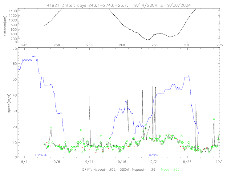
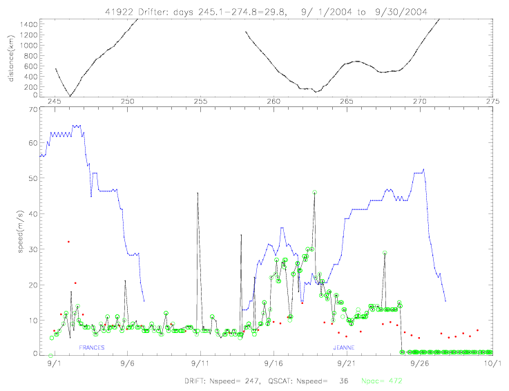 Fig. 6.1.1 Wind speed comparisons for GTS and Pacific Gyre data, for ADOS drifters (a) 41921, and (b) 41922.
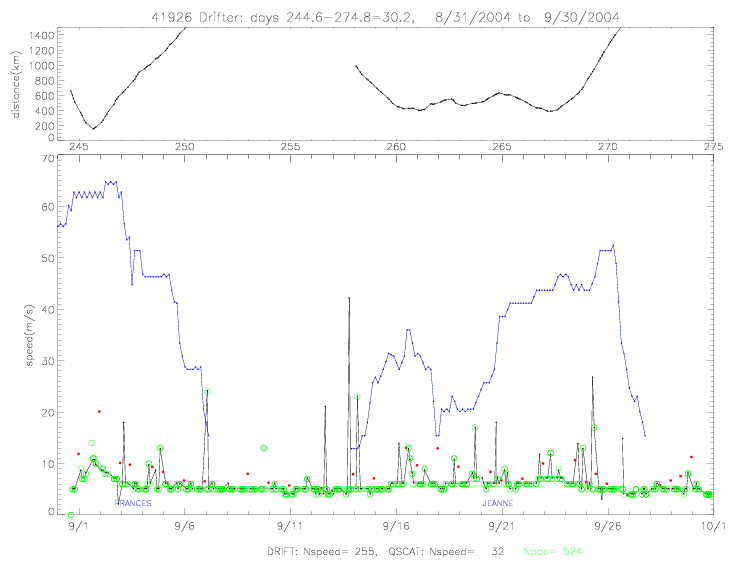 Fig. 6.1.2 Wind speed comparisons for GTS and Pacific Gyre data, for ADOS drifter 41926.
The sound pressure data from ADOS drifter 41921 is analyzed in detail, in order to derive wind
speed data. Pacific Gyre data is used as input, because it contains all transmitted data.
During each transmission 4 records of sound pressure level (spl) from four 15min sampling
intervals are transmitted. Each measurement is based on 75sec of acoustic data.
Drifter 41921 transmitted useful data from 9/4 to 10/23/2004. Sound pressure levels
for three frequency bands are presented: 0-2kHz (green), 6-10kHz (red), and 14-20kHz (blue).
The Pacific Gyre data files also contain a derived speed value (but only from the newest
15min interval in each transmission). Those values are plotted as open circles in the
upper panel of the figure 5.21. Wind speeds are computed based on the formula, which should
only be used for the 6-10kHz band:
wind speed (m/s) = { 10 (spl/20) + 104.5 } / 53.91 (Equation I)
 Fig. 6.2.1 Derived wind speed and sound pressure levels for drifter 41921, 9/4-10/23/2004.
It is clear from the above figure that the Pacific Gyre speed values are based on the 6-10kHz band.
It is also noteworthy that the sound pressure levels from all three frequency bands run almost
parallel to each. Something changes in the acoustic noise on day 281 (10/6/2004):
all frequency levels drop to lower values. This period will be scrutinized further in the
comparison with collocated QSCAT data, in order to determine if the wind regime changed or whether
the acoustic measurements cannot be trusted anymore. In the following figure, a few spikes in the 6-10kHz
band have been removed; and in order to emphasize the similarities between all three frequency bands,
the 0-2 and 14-20kHz bands have been shifted to match the 6-10kHz levels as best as possible
by using the difference in mean spl level for the entire time period shown.
 Fig. 6.2.2 Wind speed and spl; spikes removed in 6-10kHz, and shifted 0-2kHz and 14-20kHz.
Further down on this page the drifter observed wind speeds will be compared with collocated QSCAT.
This comparison will be done for the 15min data, as well as for hourly estimates.
It is useful to know that measured sound pressure levels do not change very much during four
15min intervals. In the following figure, histograms are presented for all three frequency bands
that show the distribution of differences between the four 15min measurements. When no records are
missing, there are six differences among the four values. Only 5-8% of the data have differences
larger than 5 among the four measurements per hour. This fact could be used as a quality control
measure to remove spiky measurement errors. Note that a change in spl of 5 units results in a change of wind
speed of 1.5 m/s in wind regimes of 3-5m/s, but 5m/s in wind regimes of 8-12m/s, and 8m/s in wind regimes
of 12-20m/s.
In the following figure, the number of differences ("Ndat") are listed at the top when the values
exceed the maximum plot value. When the number of data exceed 0.5%, the percentage of data
are listed as well.
 Fig. 6.2.3 Histogram of differences among, usually 4, observed sound pressure levels per 1 hour.
Comparisons with collocated QSCAT data are presented below. Because of the sampling frequency of the
drifters and the resulting time differences with local overflights of the sactterometer (see fig.3.1 & 3.2),
it was necessary to use a maximum time difference of 4hr for collocations. The maximum distance allowed
was 100km. The resulting average time difference of the collocations is ca. 140min (2:20hr); and the average
distance is 17km (ranging from 1 to 95km).
Presented are timeseries of wind speed:
drifter speeds derived from the 6-10kHz frequency and standard QSCAT. Also shown are the
wind speed differences and the time differences of the two collocated measurements. Note that the time period
after day 281 (when the relative magnitudes of the three sound channels change) does not exhibit
anomolous differences with respect to QSCAT.
 Fig. 6.2.4 Drifter 41921 6-10kHz derived wind speeds and collocated QSCAT (red dots).
Scatterplots of wind speeds from drifter and QSCAT are presented below. Rain-flagged data are marked in red.
 Fig. 6.2.5 Drifter wind speed vs. QSCAT.
The few rain-flagged data (Nrain=4) do not exhibit very large wind speed differences with respect to
QSCAT, and, therefore, will not be excluded from the comparisons.
About a third of the drifter measurements tend to overestimate wind speed. Breaking surface waves produce large
acoustic noise that result in larger measured sound levels than only due to wind speed at the surface
of the ocean. That contamination of the acoustic signal would bias the results towards higher wind
speeds.
Also plotted are scatterplots of wind speed differences vs. time differences and separation distances.
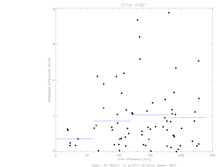
 Fig. 6.2.6 Wind speed differences vs. (a) time differences, and (b) distances.
In the time difference plot, the average speed differences
for 4 time difference (Tdif) intervals are drawn with blue lines. While the speed differences for
Tdif = 0-60min are the smallest (average=0.7m/s), the averages for longer Tdif do not change very much for
time differences from 60 to 230min (average speed differences vary between 1.7 and 2.1m/s).
Therefore, it seems reasonable to include the relatively large
time differences (up to 230min = 3:50hr) in the collocation data sets.
Distances between collocated data tend to be within 20km. The standard QSCAT product is provided on a
25x25km grid. Larger distances only occur in patches of missing QSCAT wind vector cells (WVC),or when
the drifters were at the edge of the scatterometer swath.
The next figure presents the functional fit between sound pressure level (spl) and wind speed.
Black dots indicate the wind speeds derived from Equation I (a=20., b=104.5, c=53.91). When compared with
collocated QSCAT, the average speed difference is 1.2m/s (Stdev=2.1m/s). Using the collocated
QSCAT wind speeds, one can derive an estimate of the conversion coefficients based on a
least-square-fit: a=39.21, b=1.1, c=2.84. This conversion function and the resulting wind speed
estimates are plotted in red.
The data are limited to wind speeds of less than 15m/s. For small wind speeds (< 7m/s),
the best-fit function agrees very well with the function from Equation I. For stronger winds,
the best-fit function would result in lower estimates of wind speeds.
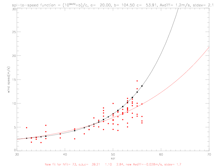 Fig. 6.2.7 Conversion function between sound pressure and wind speed.
Hourly estimates of drifter derived wind speeds are used in the following figures with
collocated QSCAT. The hourly estimates are computed by averaging only the two lowest sound
pressure levels in every hour. The wind speed satterplots show that the
correlation betwen drifter and QSCAT speeds gets better: the average speed difference drops from
1.2 to 0.6m/s, and stdev shrinks from 2.1 to 1.6m/s. Also the best-fit conversion function
moves closer to the theoretical function.
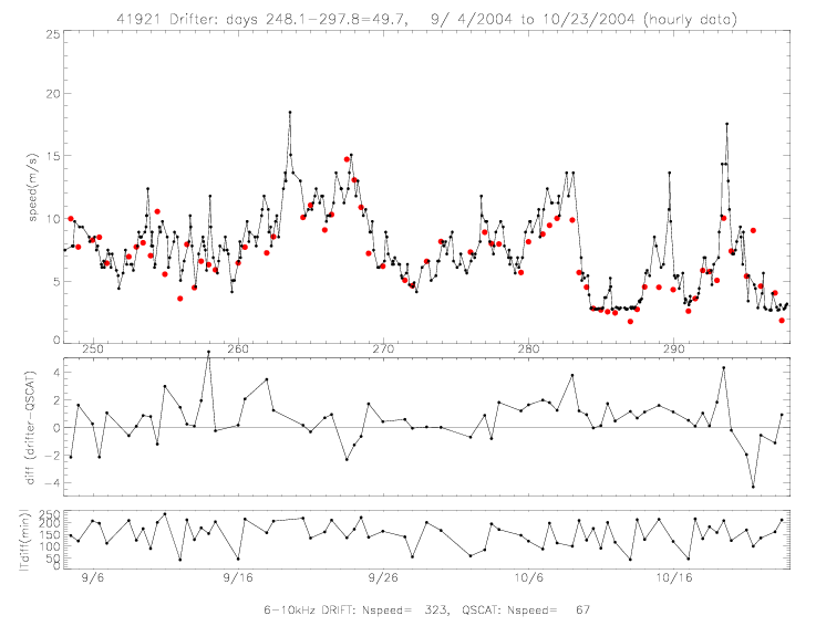 Fig. 6.2.8 Hourly drifter 6-10kHz derived wind speeds and collocated QSCAT.
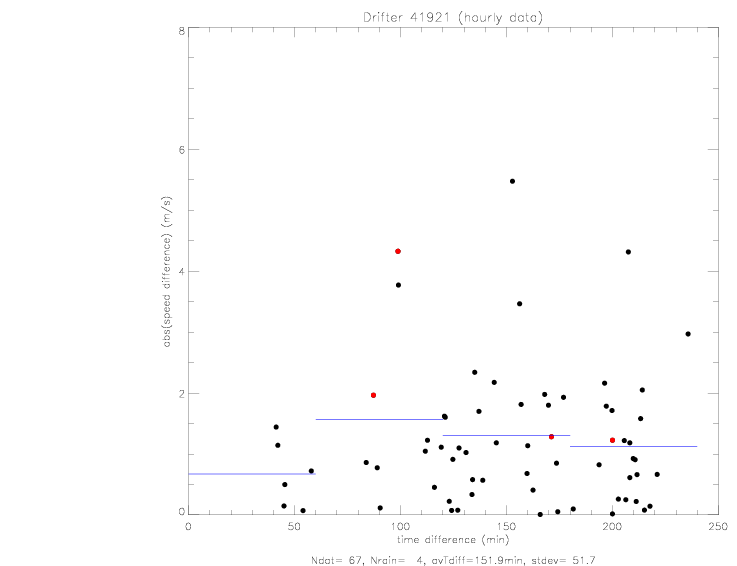
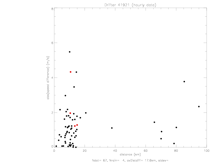 Fig. 6.2.9 Hourly wind speed differences vs. (a) time differences, and (b) distances.
From the two figures above it is easy to see that most of the speed differences have been reduced, when comparing
the hourly with the 15min data.
In particular, it is striking how speed differences within 20km separation distances have greatly been reduced.
In the 15min data, 27% (17 out of 63) of the data within 20km had speed differences of more than 2.2m/s (max=7.7m/s).
In the hourly data, this percentage has been reduced to 8% (5 out of 59, max=5.5m/s).
There are seven outliers in the hourly data set with relatively large speed differences (2.2-5.0 m/s). These outliers
are either associated with large time differences (5 with Tdif>90min) or large separation distances (1 with dist>80km).
In the next section, a sub-sample of the hourly is investigated, from which these seven outliers have been
removed.
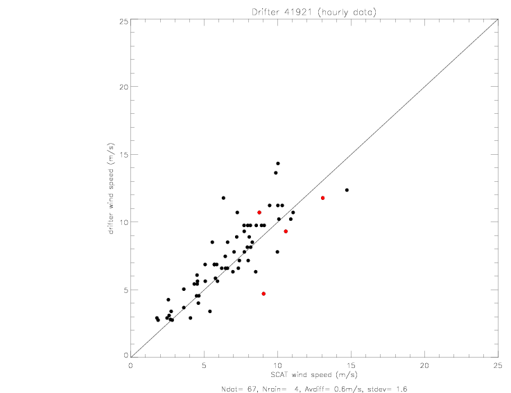
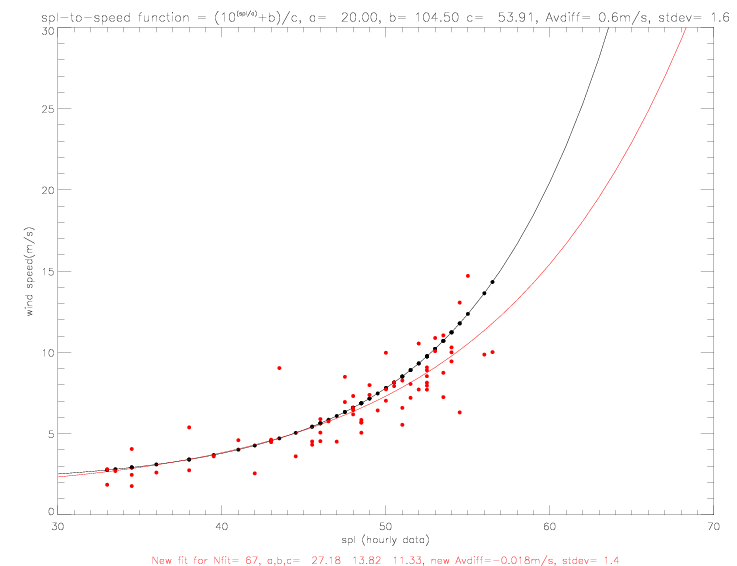 Fig. 6.2.10 (a) Hourly drifter wind speed vs. QSCAT, and (b) conversion function.
A subsample of hourly estimates is presented below. For the subsample large speed differences
with either large time differences (speed diff>2.2m/s & Tdiff>90min) or large separation distances
(speed diff>2.2m/s, and dist>80km) were eliminated (7 out of 67 samples were removed).
For the resulting 60 collocated pairs of drifter derived wind speeds and QSCAT measurements, the average speed
difference is 0.4m/s, with Stdev = 1.0m/s.
The best-fit conversion function, based on this subsample, requires coefficients of (20.3, 98.0, 53.2), for
which the theoretical values are (20.0, 104.5, 53.9). The best-fit average speed difference is 0.0m/s,
with Stdev = 1.0m/s.
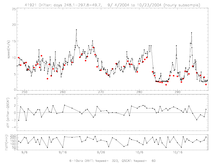 Fig. 6.2.11 Subsample of hourly drifter 6-10kHz derived wind speeds and collocated QSCAT.
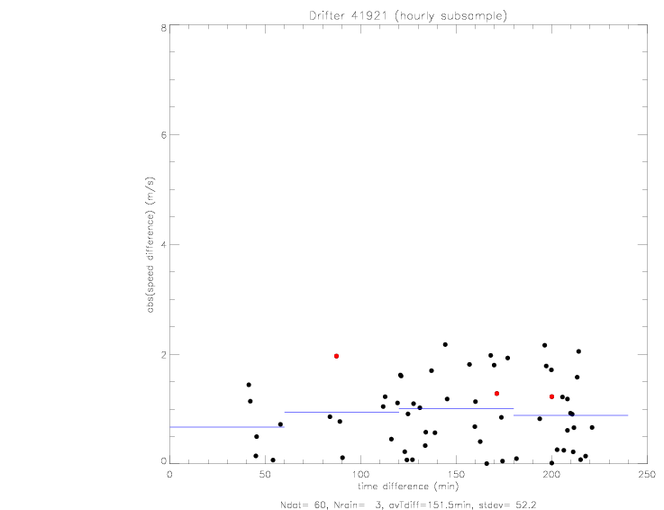
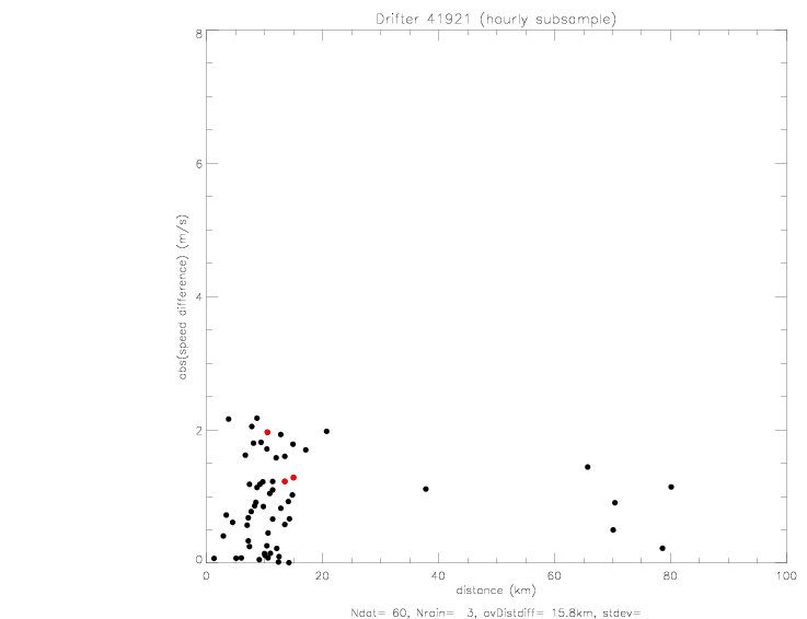 Fig. 6.2.12 Subsample of hourly wind speed differences vs. (a) time differences, and (b) distances.

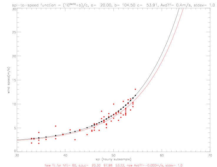 Fig. 6.2.13 (a) Subsample of hourly drifter wind speed vs. QSCAT, and (b) conversion function.
GTS wind direction data files consist only of the most recent measurement from each 1-hour measurement cycle.
The Pacific Gyre data (Pac) include all four 15-min data from each 1-hour cycle as they have been transmitted to ARGOS.
In this section, GTS data are compared with Pac data. For this comparison, the time stamps of
Pac data are not adjusted by the "age" value, which indicates the time difference between measurement time
and reception by ARGOS. Only the most recent measurements from each 1-hour sampling cycle is compared, since
GTS files do not include any other 15-min measurements. The un-adjusted Pac time stamps differ from GTS, generally,
by not not more than 4 minutes. Furthermore, in order to compare the same data, Pac data records of bin number (1-72)
is converted to wind direction by multiplying by 5° (but not subtracting 2.5°, which should be done to be exact).
The resulting values are rounded to nearest 10degrees, which reflects the accuracy of the GTS data.
Also, none of the directions are corrected for battery effect (which is required for ADOS data, and can be
as large as 34°), or for magnetic declination (9-13°).
In the following figures, Pac wind directions are plotted with black dots, GTS are in red.
GTS records with time stamps that match Pac time stamps (generally, within 4min), but which have different
direction values, are marked in blue and are counted as "Ndiff" data in the subtitle. GTS records with time
stamps that do not match any Pac time stamps, are marked in green ("Nextra"). Any black Pac values with no red mark,
indicate Pac values with no matching GTS time stamps ("PAC: Nextra").
 Fig. 6.3.1 Wind direction comparison GTS vs. Pac for ADOS drifters (a) 41920, and (b) 41922.
 Fig. 6.3.2 Wind direction comparison GTS vs. Pac for ADOS drifters (a) 41923, and (b) 41925.
The average differences and rms are calculated separately for non-rain flagged data, and rain-flagged data.
The 1:1 line is plotted, as well as the non-rain rms lines.
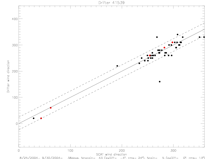
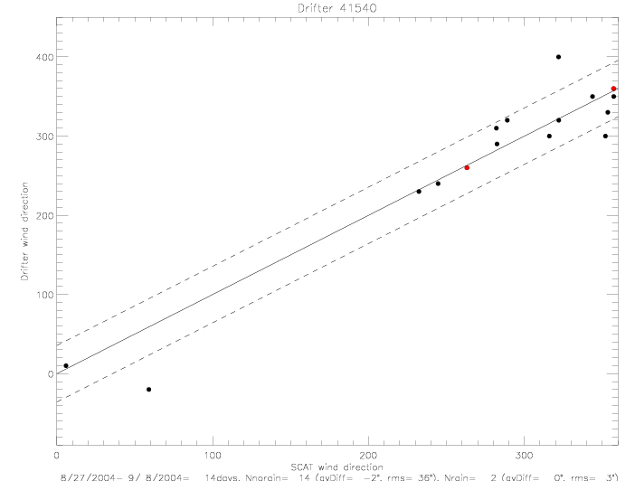 Fig. 7.1 Wind direction scatterplot for Metocean drifters (a) 41539, and (b) 41540.
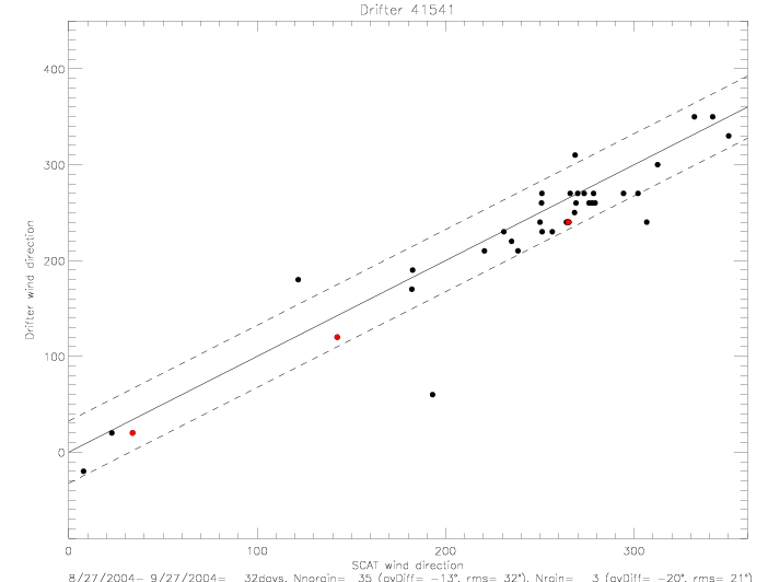
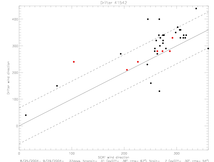 Fig. 7.2 Wind direction scatterplot for Metocean drifters (a) 41541, and (b) 41542.
 Fig. 7.3 Wind direction scatterplot for Metocean drifters (a) 41543, and (b) 41544.
 Fig. 7.4 Wind direction scatterplot for Metocean drifters (a) 41545, and (b) 41590.
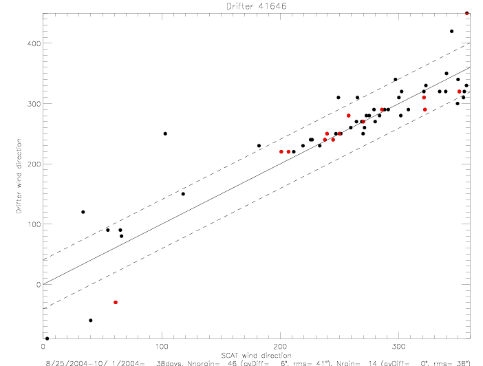 Fig. 7.5 Wind direction scatterplot for Metocean drifter 41646.
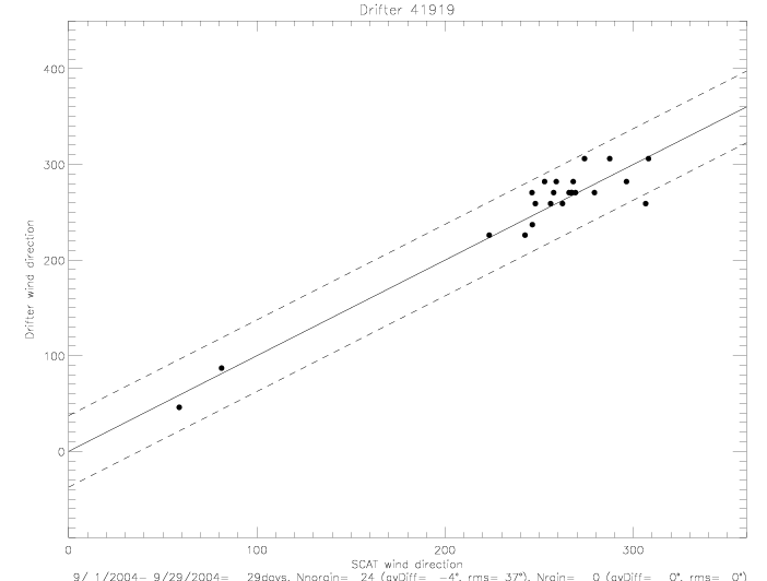
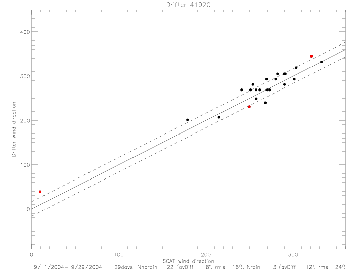 Fig. 7.6 Wind direction scatterplot for ADOS drifters (GTS data) (a) 41919, and (b) 41920.
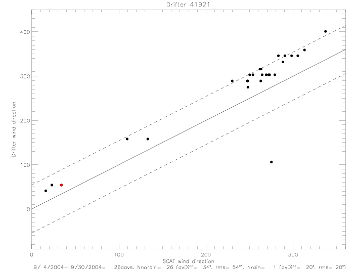
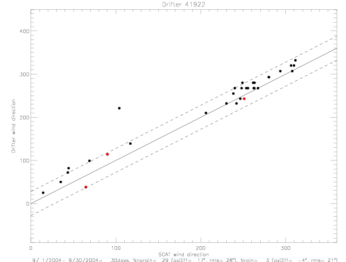 Fig. 7.7 Wind direction scatterplot for ADOS drifters (GTS data) (a) 41921, and (b) 41922.
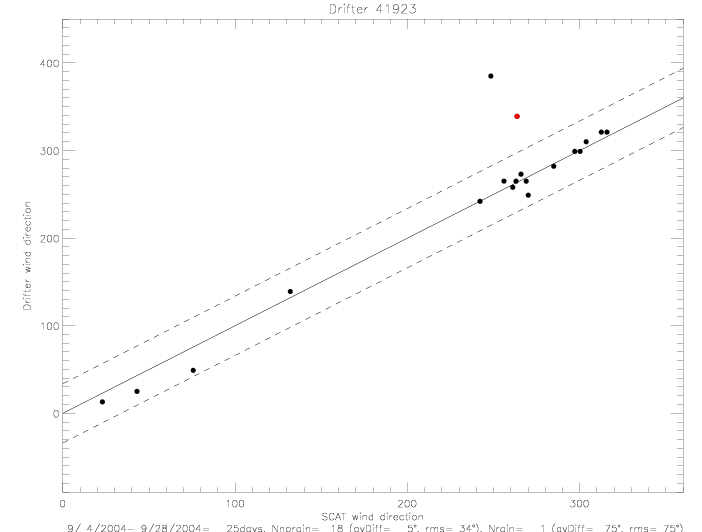
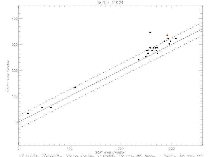 Fig. 7.8 Wind direction scatterplot for ADOS drifters (GTS data) (a) 41923, and (b) 41924.
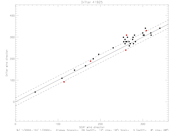
 Fig. 7.9 Wind direction scatterplot for ADOS drifters (GTS data) (a) 41925, and (b) 41926.
The above figures for ADOS wind directions are based on GTS data. The GTS data have only been corrected
for the battery effect. PACIFICGYRE data have also been used to derive wind speeds. These data include
all 15min records, not just the latest transmission as in the GTS data. PACIFICGYRE data have been corrected
for the battery effect and also for magnetic declination. The resulting scatterplots with collocated
QSCAT are presented below.
 Fig. 7.10 Wind direction scatterplot for ADOS drifters (PAC data) (a) 41919, and (b) 41920.
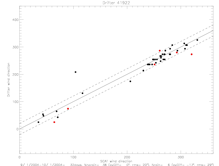 Fig. 7.11 Wind direction scatterplot for ADOS drifters (PAC data) (a) 41921, and (b) 41922.
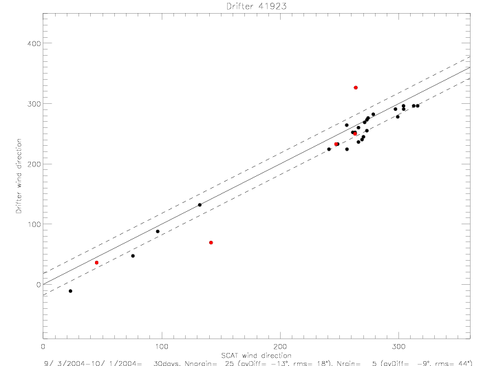
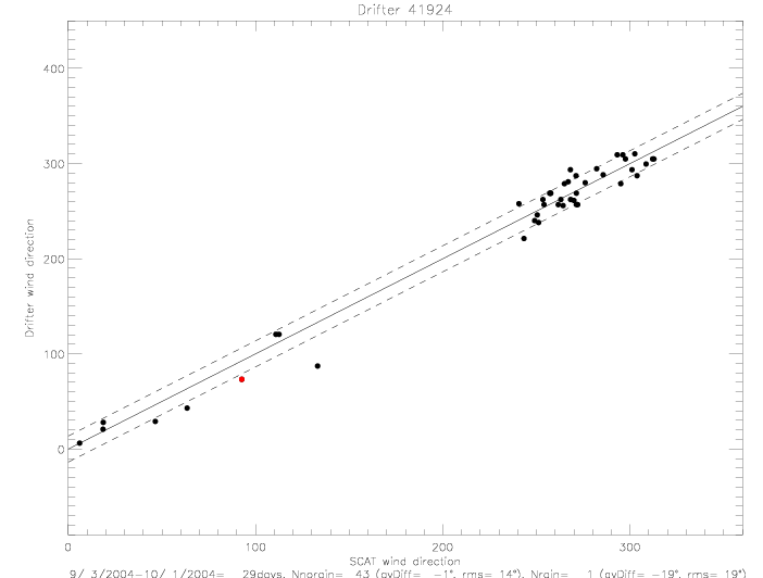 Fig. 7.12 Wind direction scatterplot for ADOS drifters (PAC data) (a) 41923, and (b) 41924.
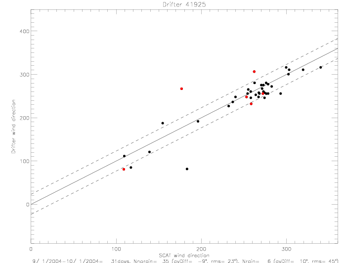
 Fig. 7.13 Wind direction scatterplot for ADOS drifters (PAC data) (a) 41925, and (b) 41926.
The average differences and rms are calculated separately for non-rain flagged data, and rain-flagged data.
The 1:1 line is plotted, as well as the non-rain rms lines. Drifters 41646, 41919, 41920, 41923, 41924, and
41925 do not have good speed data. Drifters 41921, 41922, and 41926 are questionable.
 Fig. 8.1 Wind speed scatterplot for Metocean drifters (a) 41539, and (b) 41540.
 Fig. 8.2 Wind speed scatterplot for Metocean drifters (a) 41541, and (b) 41542.
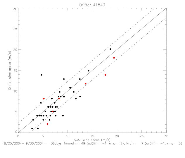
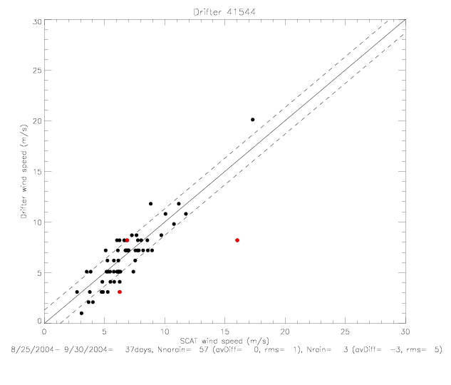 Fig. 8.3 Wind speed scatterplot for Metocean drifters (a) 41543, and (b) 41544.
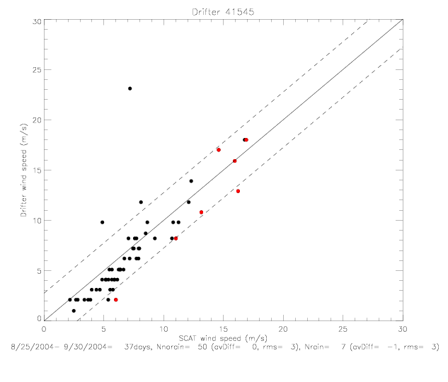
 Fig. 8.4 Wind speed scatterplot for Metocean drifters (a) 41545, and (b) 41590.
 Fig. 8.5 Wind speed scatterplot for ADOS drifters (a) 41921, and (b) 41922.
 Fig. 8.6 Wind speed scatterplot for ADOS drifter 41926.
The wind speed statistics for drifter vs. QSCAT collocations are summarized in the next table. The comparisons are
only shown for those Metocean drifter which are used to plot wind speed near the hurricane center
( Drifter data in Hurricane Momentum Equation ).
Sub-samples are generated by only including differences within two standard deviations of the average difference
of each drifter.
Table 8.1: METOCEAN collocated wind speed differences
| | No-rain data |
Sub-sample |
| Drifter | days | Ndat | av Diff | st.dev. |
Nsub | av Diff | st.dev. |
| 41539 | 38 | 51 | -1.0 | 1.7 | 49 | -1.3 | 1.0 |
| 41540 | 15 | 19 | -0.3 | 1.8 | 17 | -0.8 | 1.2 |
| 41541 | 38 | 53 | -0.4 | 3.3 | 47 | -1.5 | 1.2 |
| 41542 | 37 | 47 | -0.5 | 3.2 | 45 | -1.1 | 1.5 |
| 41543 | 38 | 49 | -0.7 | 2.2 | 48 | -0.9 | 1.7 |
| 41544 | 37 | 57 | -0.2 | 1.3 | 55 | -0.3 | 1.2 |
| 41545 | 37 | 50 | -0.4 | 2.8 | 49 | -0.7 | 1.5 |
| | | | | | | | |
| average |
| | | | | -0.9 | 1.3 |
In this section, the rapid cooling of SST due to Frances, and the slow warming of
SST during the 3 weeks after Frances are analyzed based on drifter measurements.
A subset of drifters clustered within the CBLAST region (ca. 288° - 292°E, and 21° - 25°N)
is considered. These 40 drifters consits of:
13 Minimets (41927, 41928, 41929, 41931, 41932, 41933, 41934, 41935, 41936,41937,41938,41939,41941),
6 ADOS (41919, 41920, 41922, 41924, 41925, 41926), 3 Metocean (1539, 41543, 41545),
12 SVP-100m (41617, 41618, 41619, 41620, 41622, 41623, 41668, 41669, 41671, 41852, 41853, 41854),
3 SVP-15m (41942, 41943, 41944), 2 SST (13518, 13610), and 1 SST&pres (13533).
The first 11 days after deployment, and the next 11 days are shown here.
 Fig. 9.1 Drifter tracks in CBLAST region, (a) during first 11 days, and (b) next 11 days.
For the purpose of this analysis the drifter data are interpolated 3-hourly and smoothed with
a 1-day running-average.
As an example, the smoothed SST data for ADOS drifter 41925 is shown below.
 Fig. 9.2 SST from ADOS drifter 41925, incl. 1-day smoothed data.
The following figures show maps of SST during the first 3 weeks after Frances passed over the drifters
in the CBLAST region. SST is plotted as the difference of observed SST minus the pre-Frances value at each
drifter. The IDL "Min_Curve_Surf" function was used to interpolate the irregularly gridded set of drifter
points onto a surface with "minimum curvature", at a resolution of 0.25° x 0.25°. This function does
an acceptable job of finding a reasonable SST surface. The resulting 3-hourly maps are shown for 12:00 UTC
on September 1 (just before Frances arrived), 2, 3, 4, 5, 10, 15, and 20. Printed on the plots are the drifter
SST data that went into generating each map. Each drifter location includes the last two digits of the drifter and
a letter for the drifter type: M=Minimet, m=Metocean, A=ADOS, S=SVP-100m, s=SVP-15m, p=SST&pres, t=SST.
Also shown is the track of Frances, with 3-hourly marks from 9/1 6:00hr to 9/2/04 15:00hr. On September 20, 12:00
Jeanne had already passed over the drifters and was at 26.4°N, 288.3°W, just north of the plotted
region. Its track is shown on the last map, too.
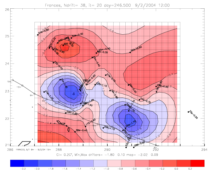 Fig. 9.3 Interpolated drifter SST change map (SST minus pre-Frances SST), for (a) 9/1/04,
and (b) 9/2/04.
Fig. 9.3 Interpolated drifter SST change map (SST minus pre-Frances SST), for (a) 9/1/04,
and (b) 9/2/04.
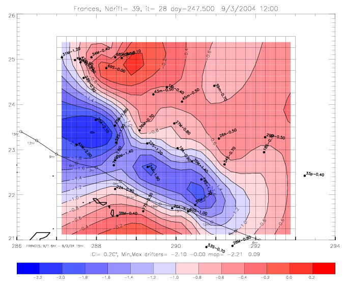
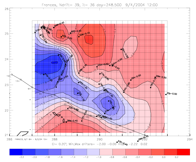 Fig. 9.4 Interpolated drifter SST change map (SST minus pre-Frances SST), for (a) 9/3/04,
and (b) 9/4/04.
Fig. 9.4 Interpolated drifter SST change map (SST minus pre-Frances SST), for (a) 9/3/04,
and (b) 9/4/04.
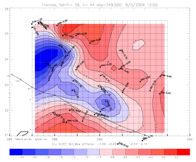
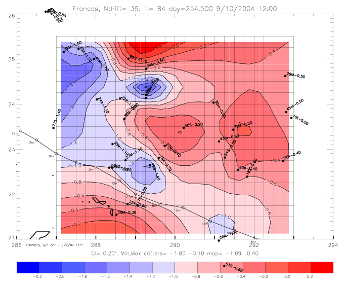 Fig. 9.5 Interpolated drifter SST change map (SST minus pre-Frances SST), for (a) 9/5/04,
and (b) 9/10/04.
Fig. 9.5 Interpolated drifter SST change map (SST minus pre-Frances SST), for (a) 9/5/04,
and (b) 9/10/04.
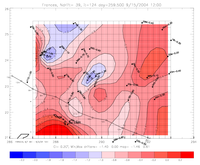
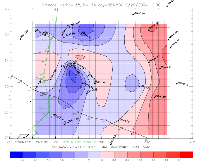 Fig. 9.6 Interpolated drifter SST change map (SST minus pre-Frances SST), for (a) 9/15/04,
and (b) 9/20/04.
Fig. 9.6 Interpolated drifter SST change map (SST minus pre-Frances SST), for (a) 9/15/04,
and (b) 9/20/04.
This interpolation scheme applies the same surface curvature in the longitudinal and
latitudinal directions. Since the SST cooling happens roughly parallel to the track of Frances, a more sophisticated
mapping routine should incorporate this preferred orientation in order to generate maps with features
more parallel to the track. For example, on Sep 2 the two regions of relatively cold SST at 288.5°W, 23°N
(coldest drifter SST=-1.8°) and 291°W, 22°N (coldest drifter SST=-1.7°) are not connected
parallel along the track of Frances (in a region with no drifter data), but instead the mapping routine
generates an area with temperatures of only -1.0°, due to drifter data of -0.8° further north of the track
(from drifter 19A-0.80 at 290°W, 23°N) and data of -0.6° south of the track (drifter 17A-0.60).
Similarly, on Sep 20 the region parallel and east of Jeanne's track, with drifter data as low as
-1.8° in two regions, are not connected along the track (through an area with no drifter observations).
Instead, the mapping function creates a small isolated area with slightly warmer SST separating the two cold regions.
The ppt file of the presentation, "Air-deployed Drifting Buoy Observations during Fabian, Isabel, Frances, and Jeanne" , can be viewed
here .
last modified on March 23, 2007
Go Back
)
)
)
)
)
)
)
)
)
)
)
)
)
)
)
)
)
)
)
)
)
)
)
)
)
)
)
)
)
)
)
)
)
)
)
)
)
)
)
)
)
)
)
)
)
)
)
)
)
)
)
)
)
)
)
)
)
)
)
)
)
)
)
)
)
)
)
)
)
)
)
)
)
)
)
)
)
)
)
)
)
)
)
)
)
)
)
)
)
)
)
)
)
)
)
)
)
)
)
)
)
)
)
)
)
)
)
)
)
)
)
)
)
)
)
)
)
)
)
)
)
)
)
)
)
)
)
)
)
)
)
)
)
)
)
)
)
)
)
)
)
)
)
)
)
)
)
)
)
)
)
)
)
)
)
)
)
)
)
)
)
)
)
)
)
)
)
)
)
)
)
)
)
)
)
)
)
)
)
)
)
)
)
)
)
)
)
)
)
)
)
)
)
)
)
)
)
)
)
)
)
)
)
)
)
)
)
)
)
)
)
)
)
)
)
)
)
)
)
)
)
)
)
)
)
)
)
)
)
)
)
)
)
)
)
)
)
)
)
)
)
)
)
)
)
)
)